

Abstract
Ever since the inception of light microscopy, the laws of physics have seemingly thwarted every attempt to visualize the processes of life at its most fundamental, sub-cellular, level. The diffraction limit has restricted our view to length scales well above 250 nm and in doing so, severely compromised our ability to gain true insights into many biological systems. Fortunately, continuous advancements in optics, electronics and mathematics have since provided the means to once again make physics work to our advantage. Even though some of the fundamental concepts enabling super-resolution light microscopy have been known for quite some time, practically feasible implementations have long remained elusive. It should therefore not come as a surprise that the 2014 Nobel Prize in Chemistry was awarded to the scientists who, each in their own way, contributed to transforming super-resolution microscopy from a technological tour de force to a staple of the biologist's toolkit. By overcoming the diffraction barrier, light microscopy could once again be established as an indispensable tool in an age where the importance of understanding life at the molecular level cannot be overstated. This review strives to provide the aspiring life science researcher with an introduction to optical microscopy, starting from the fundamental concepts governing compound and fluorescent confocal microscopy to the current state-of-the-art of super-resolution microscopy techniques and their applications.
Export citation and abstract BibTeX RIS

Original content from this work may be used under the terms of the Creative Commons Attribution 3.0 licence. Any further distribution of this work must maintain attribution to the author(s) and the title of the work, journal citation and DOI.
Introduction
A brief history of microscopy
Microscopy has revolutionized biological research. The ability to see beyond the restrictions imposed by the human eye has forever changed the way we look at nature and life. Although nobody can individually be credited for creating the first compound microscope, one of the earliest functional examples was conceived by Hans Jansen and his son, Zacharias, in the late 16th, early 17th century. Their design featured variable magnification and ultimately allowed objects to be magnified up to nine times [1, 2]. At around the same time Hans Lippershey was also working on the development microscopes, as well as telescopes, and to this day the question of who was truly first remains a matter of much contention [3].
The dawn of light microscopy in biology was ushered in by Hooke's famous manuscript 'Micrographia', published in 1665 [4]. Here, Hooke assembled a stunning collection of copperplate engravings on subjects ranging from fossils and wood to insects, all of which he observed using a handcrafted compound microscope (figure 1(A)) [4]. Some of his most famous observations are probably portrayed by the drawings of a fly's compound eye (figure 1(B)) or his depictions of plant material, using the word 'cell' to describe the individual functional units of life he observed, a first in the history of science [5].

Figure 1. Copperplate engravings from Hooke's 'Micrographia'. (A) A leather bound and gold microscope with candle light source. (B) Detailed drawing of a fly's head, clearly showing the compound eyes. In his original manuscript, Hooke annotates this drawing as the head of the drone fly. However, some contemporary entomologists believe this picture actually represents a horsefly's (Tabanus autumnalis L.) head [4, 6].
Download figure:
Standard image High-resolution imageInspired by the work of Hooke and in stark contrast with the relatively complicated dual lens designs of Jansen and Lippershey, the Dutchman Antonie van Leeuwenhoek instead opted for a single lens approach (figure 2(A)). His designs allowed him to observe specimens at magnifications up to 280 times, a feat made possible by his exceptional craftsmanship in making very small spherical lenses. His work ultimately resulted in over 500 letters written to the Royal Society describing the organisms and structures he discovered. Van Leeuwenhoek can thus be credited with the discovery of bacteria (figure 2(B)) and yeast cells, earning him the unofficial title 'father of microbiology'. He also was the first to describe red blood cells and the striated nature of muscles [7, 8].

Figure 2. Van Leeuwenhoek's microscope and its observations. (A) Hand-made single lens microscope with mechanically moving sample holder. (B) Observations of human mouth bacteria, as described by Van Leeuwenhoek in his 39th letter to the Royal Society (1683). Visible are (a) Bacillus, (b) S. sputigena and (c), (d) the path it makes, (e) micrococci, (f) L. buccalis and (g) a spirochete. Modified from Carpenter and Dallinger [9] and Lane [10].
Download figure:
Standard image High-resolution imageOver the course of the next few hundred years, microscopy evolved tremendously. Present day super-resolution microscopes are highly sophisticated instruments, featuring hundreds of optical and mechanical components. Candles have been replaced by high intensity arc-lamps, light emitting diodes (LEDs) or lasers. Images are no longer directly observed by eye but recorded using sensitive detectors and the resulting three-dimensional images are shown on computer screens. Molten glass lenses are replaced by chemically engineered glass, coated with specialized polymers. Samples are no longer mounted on needles but treated with chemicals, embedded in optically clear resins, placed on electronically stabilized stages. More often than not, everything is fully computer controlled. The amount of detail that can be visualized with modern microscopes has increased tremendously, from the micrometer to the nanometer range, and some might therefore say microscopy has evolved to nanoscopy [11]. Along with their machines, microscopists have evolved from keen observers with a talent for illustration to engineers, chemists and physicists with an interest in biology.
An optics primer
Lenses are arguably the most fundamental components of any microscope. They are often manufactured from specifically formulated glass featuring a well-defined, relatively high, refractive index (RI).
The RI is a dimensionless number that defines how a material affects light upon transmission. In a medium with an RI higher than unity, light waves will move slower compared to their speed in vacuum. Moreover, upon transition between media with different RI, light will bend or refract (figure 3(A)). This effect is wavelength dependent and can readily be observed in a relatively simple optical element such as a prism. Bending each wavelength at a slightly different angle, prisms have the ability to separate white light into its component colors, i.e. disperse it (figure 3(B)).

Figure 3. The basic concepts of refraction and lenses. (A) Refraction of a beam by a medium of higher refractive index. (B) White light dispersion by a prism. (C) The focusing of light by a convex lens.
Download figure:
Standard image High-resolution imageLenses on the other hand, refract light in such a way that it gets focused in a specific point (convex lens, figure 3(C)) or diverges (concave lens). The thickness and curvature of the lens surfaces together define the focal length.
When an object is placed at a distance further than the focal distance of a convex lens, light rays originating from any point on the object will be refracted by the lens such that they will form a real but inverted image of the object on the opposite side of the lens (figure 4(A)). This image can be observed when a screen or an imaging sensor is placed at the correct position behind the lens. The size of the image is inversely proportional to the distance of the object from the front focal point. When an object is placed exactly at, or closer than, the front focal length of a lens, refraction will cause all light rays originating from the object to travel parallel to each other or diverge upon passage through the lens (figure 4(B)). In this case, instead of a real image, a so called 'virtual' image is formed on the same side of the lens as the original object (figure 4(B)).

Figure 4. Image formation in convex lenses (A) When an object is placed in front of the front focal point (F) of a lens, an inverted real image is formed at a specific distance from the back focal point F. (B) When an object is placed at or behind the front focal point F, a virtual image of the object will be formed in front of the lens.
Download figure:
Standard image High-resolution imageThis virtual image can no longer be directly observed using a screen. Instead, an additional imaging system such as the human eye is needed. The eye possesses the ability to perceive the world because it contains a lens which projects an image of a distant object onto a biological screen, the retina, a light sensitive tissue which relays information to the brain. The size of an image on the retina is influenced by two parameters; the actual size of the object and the distance of the imaged object relative to the eye. Both parameters define the angle subtended at the eye by the object and the apparent size of the object is directly proportional to this angle (figures 5(A) and (B)).

Figure 5. Image formation in the human eye. (A) When an object is observed at a large distance, a small angle is subtended between the object and the eye, resulting in a smaller image of the object on the light sensitive element of the eye, the retina. (B) When a nearby object is observed, the subtended angle will be larger, resulting in a larger image of the object being projected onto the retina. It should be noted that the eye can change its focal length (indicated by f) by deforming its lens. This allows the human eye to focus on objects both near and far.
Download figure:
Standard image High-resolution imageIn the broadest sense, all optical instruments that magnify objects such as e.g. single lenses, operate by increasing the size of this angle, hence the term 'angular magnification' (figure 6).

Figure 6. Angular magnification by a single convex lens. (A) When an object is directly observed by the eye (eye lens, EL), a relatively small angle is subtended at the eye by the object. (B) When a simple convex lens such as e.g. a magnifying glass (M), is placed between the object and the eye, a large, virtual image will first be formed by the magnifying glass (grey image, far left). Because the eye has its own convex lens, it also has the ability to focus the diverging light rays originating from this virtual image to once again form a real image on the retina (R). Since the angle subtended by the virtual image at the eye is now much larger, a larger image of the object will form at the retina.
Download figure:
Standard image High-resolution imageTransmission microscopy
In the early days of microscopy, all instruments were 'bright field' transmission microscopes. In such microscopes, homogeneous and sufficiently intense illumination is achieved through the use of a condenser lens, which focuses light of the illumination source onto the sample. This light subsequently passes through the sample and is ultimately collected by the compound lens system of the microscope. Variations in transparency of the sample create contrast in the resulting image.
Even though modern-day instruments are often much more complex than the earliest compound microscopes, one can still grasp the essential aspects of image formation in microscopy by considering the most basic two lens system consisting of an objective lens and an ocular lens.
The objective lens typically features a very short focal length, producing an enlarged and inverted real image inside the microscope behind, or most optimally at, the focal point of the ocular. This results in a virtual image that is magnified significantly, such that it can subsequently be observed by the eye (figure 7(A)).

Figure 7. Image formation in simple lens systems in simple compound microscopes. (A) The basic two lens system of the earliest compound microscopes featured an objective lens (O) with focal points FO and FO' and an eye piece lens (E) with focal points FE and FE'. (EL) Eye lens, (R) Retina. (B) A compound microscope with a tube lens (T) features an infinity space, allowing for the introduction of additional optical elements without impact to the tube length.
Download figure:
Standard image High-resolution imageTo ensure that the objective forms an image at the focal point of the ocular lens, the relative distance between both lenses, the so-called tube length, needs to be fixed, simply because the lenses themselves have fixed focal lengths. Introduction of any additional optical element such as e.g. a (color) filter or polarizer, would change the optical path length, requiring the objective and the ocular lens to be repositioned relative to each other. Because of this, modern microscopes typically feature an additional lens inside the optical tube. This lens is aptly named the 'tube-lens' and modern objective lenses are designed such that the light rays between the objective and the tube lens are perfectly parallel, i.e. the light is focused at infinity. The tube lens is responsible for creating a real image at the ocular lens focus. This allows the section between the objective and tube lens, the infinity space, to be of arbitrary length. As such, it can cater for the relatively straightforward introduction of additional optical elements (figure 7(B)).
The imaging systems outlined here are still highly simplified. In reality, a single objective can contain more than ten individual lens elements, made from different materials, arranged into multiple groups and featuring specialized coatings. This is necessary for correcting optical aberrations that unavoidably occur when light passes through lenses. These image distortions can generally be divided into chromatic-, spherical-, coma-, stigmatic- and field curvature aberrations, which are treated in depth elsewhere [12].
Fluorescence microscopy
The fluorescence phenomenon
Fluorescence is a luminescence phenomenon where certain molecules and minerals emit light upon absorption of photons from an 'excitation' light source. Excitation to an emissive state can only occur when the wavelength of an incident photon matches the energy difference between the electronic ground state and an excited electronic state of the dye, provided that this electronic transition is also be allowed by the laws of quantum mechanics [13]. For organic fluorophores in the condensed phase, the excited molecules return to their ground energy state very shortly after the excitation event, i.e. on nanosecond time scales. Emitted photons feature a longer wavelength compared to the corresponding excitation photons. This red shift of the fluorescence emission, the 'Stokes shift', is caused by the fact that excited molecules lose a small amount of the absorbed energy through non-radiative processes such as molecular vibrations or interactions with surrounding media, i.e. heat dissipation. The radiative energy transition will therefore be smaller and, in accordance with Planck's law, the wavelength of emission will be longer (figure 8) [13]. It should be noted that not every photon absorbed by a fluorophore gets re-emitted as a fluorescence photon. The quantum yield of Fluorescence, ΦF, is the ratio of photons absorbed to photons emitted through fluorescence. As the fluorophore interacts with its surroundings, a number of other de-excitation processes can compete with fluorescence emission [13, 14]. As such, ΦF is typically lower than unity.

Figure 8. (A) Jablonski diagram showing the energy transitions in fluorescence. Upon excitation, the molecule will be in a higher vibrational state. Prior to emission, the molecule will relax non radiatively, after which emission can take place. (B) A Franck–Condon energy diagram shows how transitions can occur to different vibrational levels, resulting in characteristic shapes for the excitation and emission spectra. (C) Excitation and emission spectra typically resemble each other's mirror image because similar transitions occur with the same probability.
Download figure:
Standard image High-resolution imageBefore the advent of super-resolution microscopy, most fluorescence imaging and microscopy could be expected to occur under conditions where the excitation rate from the ground state S0 to the first excited state S1 would be lower than the radiative decay rate from S1 to S0. These conditions are said to be non-saturating. With a significant fraction of fluorophores in the ground state, the probability that processes, other than normal fluorescence decay take place from S1, is relatively small [15]. Nonetheless, competing pathways resulting in the formation of metastable dark states such intersystem crossing (ISC) from S1 to the triplet T1 or formation of radical states  or
or  are possible. Depending on e.g. the surrounding medium, these states can feature lifetimes in the microsecond to second range (figure 9(A)) [16].

Figure 9. Jablonski diagrams showing processes that compete with fluorescence emission. (A) At low excitation powers, the excited S1 state might convert to a longer lived and dark triplet state (T1) or to various other dark states, as indicated by 'D'. (B) At increasing excitation powers, transitions to higher excited states also become prevalent.
Download figure:
Standard image High-resolution imageMoreover, at increasing power levels, excitation from S1 and T1 into higher excited states Sn and Tn will also become more prevalent (figure 9(B). What is important is that all these excited states can be precursors to permanent photobleaching, resulting in irreversible loss of the ability to emit fluorescence light [15]. This probability of any of these processes resulting in actual photobleaching is quantified as the photobleaching quantum yield, ΦD, representing the number of photons that can be absorbed (and emitted) before the molecule bleaches. For low to moderate excitation powers, and well-defined chemical environments, it's value can be considered constant. However, as will become apparent in the remainder of this manuscript, many super-resolution modalities, notably SIM and STED by definition will not operate under these conditions. These techniques specifically rely on illumination intensities that are such that fluorescence brightness no longer increases linearly to the excitation intensity and photobleaching can become a significant concern.
Epifluorescence microscopes
In fluorescence microscopy, fluorophores can be excited in any number of ways, ranging from voltaic arc lamps to LED's and lasers. In general, high intensity illumination is preferred to ultimately ensure generation of sufficient fluorescent photons. While many optical arrangements exist, so called 'epi'-fluorescence microscopy, where a single lens acts as both the condenser and objective, is by far the most frequently used implementation (figure 10). For practical reasons, this lens is most often placed underneath the sample, the so called 'inverted configuration'.

Figure 10. Schematic representation of a typical fluorescence microscope and its essential components. Key is the combination of an excitation filter, dichroic mirror and emission filter, often termed a filter-cube. This combination ensures that excitation and emission light can be separated and the latter relayed to the observer.
Download figure:
Standard image High-resolution imageIn contrast with a transmission microscope, most of the excitation light in an (inverted) epi-fluorescence microscope is not absorbed by the sample and simply passes through, never reaching the detector (figure 10). Moreover, due to back scattering some of the excitation light will nevertheless be collected by the objective lens. Therefore, proper separation of excitation and emission light on their way to and from the sample, is highly important. A dedicated optical element, the dichroic mirror, is used to achieve this. It is placed in the beam path a 45° angle and reflects excitation light towards the sample but will allow the resulting fluorescent light, which is of a longer wavelength, to pass through to the detector (figure 10). A small fraction of back scattered excitation light might still be transmitted by the dichroic mirror but it is blocked by an emission filter, before it can reach the detector. This way, emission and excitation light can be completely separated (figure 10). The ability to create filters that allow one or more precisely defined wavelength bands to pass, while efficiently blocking all other light, is central to all fluorescence microscopy studies of complex biological phenomena as it enables simultaneous observation of multiple, distinctly colored species.
Fluorescence microscopy offers many benefits over transmission microscopy in biological applications. Indeed, fluorescent labels attached to the structures of interest will be visible as bright point emitters against a vast dark background, like stars in the night sky, drastically improving contrast. Furthermore, strategies for selectively linking fluorescent dyes to their target molecules in a highly specific manner are readily available (vide infra) and a lot of efforts are directed towards chemical and/or biological design of fluorophores. Indeed, careful tuning of the photophysical and (bio)functional properties of fluorescent labels has become an indispensable aspect of high resolution imaging of biological samples, as will become clear in the following sections.
Confocal laser scanning microscopy
One of the most important innovations in fluorescence microscopy, particularly for life science applications, might well be the invention of the confocal microscope. Although patented in 1957 by Marvin Minsky of Harvard University, it would take around 20 years before it could be implemented practically [17].
All microscope arrangements discussed up to this point are 'wide-field' (WF) microscopes, where the entire sample volume is illuminated at the same time. By contrast, in a confocal microscope, light is focused into a relatively small volume within a three-dimensional sample. The emission from this focal volume is collected by the objective lens, as it normally would. However, instead of recording it using an imaging device such as the human eye or a camera, it is relayed to a light sensitive point detector such as a photomultiplier tube (PMT) or an even more sensitive avalanche photon detector (APD). Although technically distinct, both PMTs and APDs convert the incident photons into an electrical signal which can be amplified, by many orders of magnitude, resulting in enhanced contrast. More in-depth discussions on photon detectors for CLSM can be found elsewhere [14].
To properly observe a sample that is many times larger than the single illumination volume, either the sample or the illumination volume need to be moved across the sample in discrete steps. The latter approach, called confocal laser scanning confocal microscopy (CLSM), is by far the most common approach in biology applications. In CLSM, a set of movable mirrors is used to direct the illumination spot. A computer collects the detector signal throughout the scanning procedure and digitally reconstructs an image from the recorded information.
The most important feature of a confocal microscope is the pinhole placed in front of the detector at a specific distance, the confocal plane. This pinhole will attenuate all light which does not originate from the focal volume, thus removing out of focus emission and greatly enhancing signal-to-noise ration and contrast (figure 11).

Figure 11. Schematic representation of confocal detection. Light originating from outside of the current focal position (blue) will be blocked by the pinhole whereas light (red) from the focal plane will be allowed to pass.
Download figure:
Standard image High-resolution imageBecause emission is only observed from a relatively thin axial section of the sample, thicker samples can also be optically sectioned. By moving the illumination spot axially as well as laterally, three-dimensional structures such as biological tissues or even whole animals can be imaged. Further developments, i.e. water immersion objectives, microscope mounted incubators and objective lens heaters even enable the observation of live samples over extended periods of time [14]. For these reasons CLSM became extremely popular in the biological and biomedical sciences.
Over time, many variations on the basic confocal design were developed such as the spinning disk confocal microscope and non-linear confocal imaging methods such as 2-photon imaging. An exhaustive review of all these variations is beyond the scope of this review but excellent sources on these topics exist [14].
Resolving power
The resolving power or resolution of an optical imaging system, is defined as the smallest distance between two points for which both these points can still be distinguished. To a certain extent, resolution can be improved through careful design of lenses and optics. However, a physical limit will ultimately be reached, deeply rooted in the fundamental laws governing light diffraction. This implies that any optical microscope has a finite resolution and this physical limit is generally referred the 'diffraction limit'.
Diffraction
The basic mechanism of diffraction is often demonstrated with the so called 'single-slit' experiment. Here, a coherent light source such as e.g. a laser is sent through a small aperture such as a linear slit or a pinhole. In a coherent light source, there is no phase difference between individual light waves, that is to say, the amplitude maxima of individual waves are aligned in time and space (figure 12(A)). As such, they are often represented as plane waves where each wave front corresponds to the spatio-temporal position of the wave maxima (figure 12(A)).

Figure 12. (A) In coherent light, there is no phase difference between individual light waves. (B) Coherent light can be represented as a plan wave. Here in effect, each plane corresponds to the spatial position of the maxima of coherent light waves. Schematic representation of the diffraction patterns generated by the different aperture geometries. (C) A single slit aperture yielding a striped diffraction pattern. (D) A circular aperture yielding an Airy pattern.
Download figure:
Standard image High-resolution imageAs the waves propagate, the wave fronts move along the direction of propagation. When a planar wave front encounters an infinitesimally small slit, it will be converted to a perfectly cylindrical wave front as the slit itself will behave as though it was a point source [12]. As the size of the slit is increased, every point along its width will similarly act as a point source and the individual wave fronts originating from these points will start to interfere, generating characteristic diffraction patterns (figures 12(B), (C)). Similarly, when light originating from a point object is relayed by a microscope, the lens will act as a circular aperture. By the time the light reaches the camera, diffraction will thus cause the light coming from the original point to be spread out, causing that single point source to be imaged as a distinctive concentric geometrical pattern, aptly named the 'point spread function' (PSF) (figure 12(D)). When projected onto the image plane, this PSF can be seen as a bright circle surrounded by alternating dark and bright concentric rings. This pattern was first described by George Bidell Airy in the 19th century and is therefore commonly known as the Airy function or Airy pattern. The central region of this pattern is referred to as the 'Airy-disk' (figure 12(D)) [12]. Intuitively, resolution can be defined as the distance between two partially overlapping Airy patterns such that they can still be distinguished as separate entities.
The exact properties of the point spread function, the diameter of the Airy disk and thus ultimately the resolution, are governed by the wavelength of the light and the characteristics of the microscope, in particular the efficiency of its lenses to capture light.
Numerical aperture and resolution
A formal treatment of resolution requires introduction of the concept 'numerical aperture':

Here, f is the focal length of the lens and D the diameter of the entrance pupil. The numerical aperture is a dimensionless number that quantifies the ability of an objective to capture light. As more light is captured, the obtained PSF will approach the actual size of the imaged point. This explains why high-quality microscopes, telescopes and cameras all require large diameter lenses to resolve more details and ultimately yield high resolution imagery.
However, mere inclusion of a high NA objective in a microscope is not enough to obtain well resolved images. Indeed, as light travels from an emitter in a biological sample toward the objective, it will encounter media with different refractive indices, i.e. tissue or intracellular medium, buffers with different solutes, carrier glass and air. At each phase boundary, some of the light is reflected whereas the rest is refracted along the optical path. This will unavoidably result in a loss of photons and ultimately resolution, even if a high NA objective is used. Whereas it might be hard or even impossible to prevent losses in the sample itself, 'immersion' liquids are typically used to replace the air between the carrier glass and the objective to prevent losses at this boundary. Various types of liquid can be used, ranging from water to e.g. mineral or organic oils, all of which will feature a refractive index higher than air. The optimal choice of liquid depends on the NA of the objective but in all cases, this 'matching' of the refractive index between the carrier and objective will result in a reduction of light losses, allowing the light capturing potential of a high NA objective to be maximized.
When considering immersion liquids, NA can be expressed as:

with η the refractive index of the immersion medium and 'θ' the angle of the cone over which the objective can capture light from the sample. The angle of the cone is defined by the focal length of the objective (the closer the sample is to the objective, the wider the cone). In air (η = 1) the angle of the cone (θ) for typical objectives ranges from 15° (20X objective) to 72° (100X objective), giving the objectives an NA of 0.25 to 0.95 respectively. Indeed, 0.95 is the maximum obtainable NA of an air objective. When using certain oils as an immersion medium (η ≈ 1.45) with an 100X objective (with a focal length yielding a 72° conus angle) the resulting NA is around 1.4 [14]. This is practically speaking the highest routinely achievable NA in microscopy when using only a single objective (also see: 4Pi and InM microscopy).
In 1873 the physicist Ernst Abbe empirically defined the resolution of a microscope in terms of the NA of an objective lens as follows:

Here, d is the minimum distance between 2 points that can still be resolved and λ the wavelength of the observed light. The visible spectrum approximately ranges from 400 (blue) to 750 (deep red) nanometer and the typical oil immersion objective has an NA of 1.4. On average, this results in a maximum resolution of around 200 nm for a typical microscope and this physical resolution limit, also known as the diffraction limit, remained unchallenged for hundreds of years.
An alternative treatment of resolution was put forth by Lord John William Strutt, Baron of Rayleigh, who won the Nobel prize in Physics in 1906. He stated that two-point light sources of identical intensity could be resolved by the human eye if the Airy disk of one point does not come closer than the first minimum of the second point's Airy function (figure 13). This realization led him to formulate his own definition of resolution:


Figure 13. Overlap of Airy functions defines the resolution. Rayleigh calculated that a ±20% decreases in intensity can be resolved by the human eye. This corresponds with the overlap of the Airy disk of one Airy functions with the first minima of the second Airy function. At the left two resolved Airy functions are shown, while at the right two unresolved Airy functions can be seen. The middle represents two Airy functions separated by the Rayleigh limit.
Download figure:
Standard image High-resolution imageHere, D is the lens aperture [12]. When this condition is met, a visible decrease of intensity of around 20% will occur between two partially overlapping Airy-disks. It should be mentioned that 'clearly be resolved by the human eye' is of course a very subjective measure, as Hecht and Zajac noted in their widely known book 'Optics' [12]:
'We can certainly do a bit better than this, but Rayleigh's criterion, however arbitrary, has the virtue of being particularly uncomplicated'.
In conclusion, and despite its limitations, the following expression, modified from both the Abbe and Rayleigh criteria, is still widely accepted as a fitting compromise between different mathematical treatment of lateral resolution of a wide-field fluorescence microscope:

Lateral, axial and temporal resolution of confocal systems
To appreciate what determines resolution in a confocal microscope, first consider a laser scanning microscope without pinhole. When the point-like source gets scanned across the sample, its point-like nature is not maintained upon transfer through the microscope optics. Instead, at the sample, the illumination source will appear as an intensity distribution, i.e. point spread function of illumination (PSFill). The properties of this PSF are once again determined by the characteristics of the optics and the wavelength of the illumination light. After excitation by PSFill, point emitters in the sample are imaged as a PSF (PSFdet) at the detector [18].
Each recorded signal in a confocal acquisition can effectively be viewed as the result of two independent events, each occurring with a certain probability. First, an illumination photon needs to reach a point p(x, y, z) in the sample with the spatial distribution of photons at the sample represented by PSFill. PSFill can effectively be considered as a probability distribution hill(x, y, z). Next, the emitted fluorescence photon arrives at the detector according to PSFdet. The probability of this happening is given by hdet(x, y, z) [18]. The probability of detecting a signal is therefore determined by the product of both probability distributions [18]:

This has important consequences when considering the resolution of confocal systems. Firstly, as discussed previously, the width of PSFill and PSFdet is directly proportional to λill and λdet respectively. For a typical dye like fluorescein isothiocyanate (FITC) the Stokes shift results in a difference of 17 nm between λill and λdet, amounting to a ratio of 505 nm/488 nm = 1.05. In other words, PSFill is 5% narrower than PSFdet, resulting in a minor resolution increase. However, for most typically used dyes, this effect is so small that the previous equation can be re-written as:

Considering that the square of a probability distribution is narrower than the original distribution, it becomes easy to appreciate how a confocal system will be able to provide better resolution compared to a wide field microscope, even in the absence of a detection pinhole (figure 14(A)).

Figure 14. (A) When two identical PSFs are multiplied, the resulting product will be narrower. (B) Resolution improvement in confocal microscopy. In wide field microscopy, illumination of the entire field-of-view at once will inherently result in closely spaced emitters to be imaged as overlapping PSFs. When scanning the same sample with confocal microscopy, the points can be separated better. The Gaussian intensity profile of the confocal spot will excite molecules most efficiently near the maximum of the illumination PSF and much less so near its edges. By scanning an image in this way contrast, and thus resolution, is increased.
Download figure:
Standard image High-resolution imageAnother, perhaps more intuitive, way to appreciate the resolution advantage offered by CLSM is found by considering how point scanning affects sample illumination. Indeed, during scanning, the sample is not illuminated throughout with the same intensity, as is the case in wide-field microscopy. When two fluorescent points are spaced close together and the laser beam passes them, they will both have the same brightness only when the laser beam is positioned exactly between them. In other cases, when the laser beam is centered respectively on the first or second point, they will exhibit different fluorescent intensities. A fluorescent point illuminated by the edge of the confocal volume will emit less light because it is excited with less photons and will thus contribute less to the total signal for that coordinate. This will cause the average intensity drop between the two points to be more pronounced in the final image, i.e. point scanning illumination improves contrast, even in the absence of a detection pinhole. (figure 14(B)).
Of course, in practice, confocal systems do feature a detection pinhole. In addition to blocking out-of-focus light, it has further beneficial effects on overall image contrast. Pinhole size (PH) in a confocal microscope is typically expressed in Airy units (AU). Here, one AU is the diameter of the central Airy disk of a point emitter visualized by the system. The Airy unit is a wavelength dependent property. The pinhole diameter is reduced such that only light originating from the central disk of the Airy pattern can pass, blocking the peripheral rings, enhancing contrast between closely spaced emitters. However, extreme reductions of the pinhole diameter would result in exceedingly poor signal to noise ratios which would offset any gain in contrast. Therefore, a pinhole size of 0.25 AU is considered a practical lower limit. Here, the illumination PSF and the detection PSF almost completely overlap (figure 15).

Figure 15. The effect of the pinhole on resolution in a confocal microscope. In a confocal system, both the excitation PSF (cyan) and the detection PSF (green) need to be taken into account. The PSFs are represented here by their FWHM-boundaries. When the pinhole is wide open (left), Both the focused laser beam yields PSFill and a point emitter is results in PSFdet, both PSFs are limited by diffraction and PSFdet is wider due to the effect of wavelength. When the pinhole size is reduced to approximately 0.25 AU, both excitation and emission PSF can be made to match in size.
Download figure:
Standard image High-resolution imageIn conclusion, confocal laser scanning microscopy offers an increased resolution to normal fluorescence microscopy. Especially its ability to section thicker biological samples, without significant resolution impairment due to out-of-focus fluorescence, is a huge improvement. The achieved lateral resolution enhancement is modest but significant, although it is highly dependent on the sample labeling conditions. Bright labels can be used to image with higher resolution than relative dimmer labels, as the number of emitted photons is of critical importance to make up for a decreased pinhole size. As a rule of thumb, we could say confocal microscopy is inherently capable of slightly improving the resolution compared to conventional microscopy. Closing the pinhole maximally adds an additional improvement factor of √2 (≈30%). When we approximate the lateral resolution limit of conventional microscopy to 250 nm, we could approximate the lateral resolution of confocal microscopy to around 180 nm. Unfortunately this improvement is rarely fully achieved, as there are not an unlimited amount of fluorescent photons available in real biological samples and empirical resolutions are often closer to 250 nm [19]. Furthermore, temporal resolution is decreased, as each pixel needs to be imaged sequentially.
Sampling in digital microscopy
Since the time of Abbe and Rayleigh, microscopy has been digitized and optical limitations are no longer the sole determinants of the resolution. The human eye has largely been supplanted by electronic point detectors or camera sensors. All of which sample continuous image data as a discrete grid of pixels, i.e. a bitmap. Each pixel in a digital image covers a specific area of the sample and the average intensity of light originating from that area is typically represented by an integral value.
In the ideal case, the number of pixels in a digital image would be infinitely large and the physical area represented by each pixel would be infinitesimally small. This way, no information would be lost in the sampling process and resolution of the final image would only be limited by optics. If on the other hand, only a single pixel would be used to represent all the information contained within the field of view of a microscope, the image would just be a grey plane. The only information that could be recorded in this case would be the average intensity of the sample.
In light of these considerations it becomes apparent that proper choice of pixel numbers and their size is instrumental to maximizing the full resolving power of a microscope. Here, the Nyquist-Shannon sampling theorem dictates that a continuous analog signal should be oversampled by at least a factor of two to obtain an accurate digital representation [14]. Therefore, to image with a resolution of e.g. 250 nanometers, pixels should be smaller than 125 nanometers. This way, the intensity drop between two overlapping Airy functions can be detected as to satisfy the Rayleigh criterion (figure 16).

Figure 16. Nyquist sampling in digitized confocal microscopy. (A) When point emitters are imaged by CLSM, their detected PSF is recorded. The Shannon-Nyquist criterion states that to adequately represent a PSF in a digital manner, at least 4 by 4 pixels are required. Each point emitter is scanned multiple times, as the scanning beam only moves one pixel to the right each scan step and 1 pixel down each scan line. This produces a pixelated version of the PSF (bottom left). Oversampling and computational smoothing can then give a detailed representation of the actual PSF, when we resample the 4 by 4 array on a higher resolution screen (bottom right). (B) The Shannon-Nyquist criterion allows for accurate fitting of the overlapped digitized PSFs and separating them by the Rayleigh-criterion [14].
Download figure:
Standard image High-resolution imageOne could always use more pixels than needed according to the theorem, i.e. oversample. However, a point emitter only emits a finite number of photons, spreading these out over too many pixels would ultimately render them indistinguishable from the noise level. A more comprehensive treatment of the issues involved in digital image recording can be found elsewhere [14, 19].
Finally, advancements in computer technology have made it practically feasible to use mathematical analysis to recover additional contrast and ultimately resolution. Briefly, prior to imaging, one can record an image of an isolated, sub diffraction limit feature such as a fluorescent nanoparticle. This image will represent the PSF of that microscope and it can subsequently be used to enhance recorded images through an approach called 'deconvolution' [14].
Super-resolution microscopy
A brief history
While the resolution offered by a typical wide-field or confocal microscope might be sufficient to study e.g. tissue morphology or whole-cell dynamics, many sub-cellular structures and processes remain elusive, obscured from view by the diffraction limit. Fortunately, in the past two decades, a number of pioneering scientists have strived to find cracks in this seemingly impenetrable barrier. The late Matt Gustafsson, one of the frontrunners in those early days [20], explained it as follows:
'Even though the classical resolution limits are imposed by physical law, they can, in fact, be exceeded. There are loopholes in the law or, more precisely, the limitations are true only under certain assumptions. Three particularly important assumptions are that observation takes place in the conventional geometry in which light is collected by a single objective lens; that the excitation light is uniform throughout the sample; and that fluorescence takes place through normal, linear absorption and emission of a single photon [21].'
In 2000, Gustafsson put these ideas into practice by demonstrating how controlled modulation of the excitation light, as opposed to using uniform illumination, could result in a two-fold enhancement of lateral resolution [22]. His original approach, dubbed structured illumination microscopy (SIM), has since been surpassed by many others in terms of absolute resolution, but its speed still makes it inherently suited for the imaging of highly dynamic biological systems.
Gustafsson was by no means the first to realize that it might be necessary to forego the basic operating concepts of the fluorescence microscope, which had remained virtually unchanged for decades. In the early 90s, Stefan Hell postulated that samples could be observed by two opposing objectives. The resolving power of each objective is ultimately limited by a maximum theoretical aperture angle of 2π, a value which is even lower in practice (vide supra). Combined however, they allow imaging at a 4π (4Pi) aperture angle, resulting in significantly enhanced axial resolutions [23]. Even so, 4Pi microscopy was still very much governed by diffraction. Hell understood that, in order to truly push beyond the limitations imposed by Abbe's law, he should also manipulate the behavior of the fluorophores themselves. He subsequently developed methods to switch off all but the centermost fluorophores in the diffraction limited illumination volume of a laser scanning microscope, resulting in stimulated emission depletion microscopy (STED) in 2000 [24].
Both SIM and STED are ensemble techniques, at any given time, emission of multiple fluorophores is observed. By contrast, around the same time that Stephan Hell conceived the idea for 4Pi, William E. Moerner famously demonstrated it was possible to measure the absorption spectrum of single pentacene molecules in condensed matter, albeit at cryogenic temperatures [25]. This seminal work spawned an entirely new field of single molecule spectroscopy and in a later study, Moerner would go on to show how certain mutants of green fluorescent protein (GFP) showed remarkable 'blinking' behavior in their individual fluorescence emission. Intriguingly, after several rounds of blinking, these molecules would inadvertently go into a stable dark state from which they could be recovered by a short burst of UV irradiation [26]. The year was 1997 and with his observations on GFP photo blinking behavior, Moerner had unwittingly provided Eric Betzig the means to materialize his own ideas.
Indeed, two years prior, Betzig had proposed a concept that would allow resolution enhancement through the localization, with sub-diffraction limit precision, of individual emitters in a sufficiently sparse population [27]. Betzig had originally proposed to achieve the required sparsity by spectrally separating sub populations of emitters. However, selective activation of limited numbers of fluorophores, followed by their localization and subsequent return to the dark state would prove a much more tractable approach. Together with biologist Jennifer Lippincott-Schwartz, he leveraged the controlled on-off switching of fluorescent proteins as discovered by Moerner, to demonstrate photo activation localization microscopy for super resolved imaging in biological samples [28].
The stories of the scientists who were at the forefront in those early days not only provides for an interesting read but it also shows how the field of super-resolution imaging came to be through a combination of serendipity and above all, perseverence [29]. In a time where conventional wisdom dictated their ideas might not be feasible, sometimes without proper funding, these scientists pushed on, paving the road for an entirely new field [29]. It is therefore not surprising that Eric Betzig, Stefan Hell and William E. Moerner were awarded the 2014 Nobel prize in Chemistry.
4Pi and InM microscopy
4Pi and InM are dual objective approaches to super-resolution imaging respectively developed by Hell[23] and Gustafsson [30]. Both leverage interference phenomena to increase the axial resolution of imaging. While 4Pi is a confocal laser scanning approach, InM can be considered its wide-field counterpart (figure 17). Both techniques feature a number of 'subtypes' which essentially differ by the light path in which interference is allowed to take place, being the excitation path (4Pi-A, I3M), the emission path (4Pi-B, I2M) or both (4Pi-C, I5M). These subtypes are not so much independent implementations but rather a reflection of the development process of 4Pi and InM.

Figure 17. Schematic comparison between 4Pi(C) and I5M. Both techniques use a dual objective lens configuration (O1 & O2) which flank the sample. In 4Pi the light is focused on the sample, while I5M uses wide field illumination. The emission is then collected by both objectives, thus increasing the effective aperture, before it is send to either a point (APD) or array (CCD) detector. Adapted from Bewersdorf et al [31].
Download figure:
Standard image High-resolution imageAt the time when Gustafsson developed InM, biological imaging was dominated largely by CSLM as these instruments were readily available and offered slightly enhanced lateral resolution in addition to its inherent optical sectioning capabilities (vide supra) [30]. However, computer based post processing of images acquired on wide-field instruments, so called 'deconvolution', could be shown to equally add optical sectioning capabilities to wide-field instruments. Deconvolution separates out of focus light from the actual in plane information [32]. Similar computational approaches are also applied in interference imaging microscopy (I2M). Here, emission is collected from two opposing objectives instead of just one. If care is taken such that both light paths are equal in length, an interference pattern will be generated on the CCD camera sensor. While this does not result in directly viewable images, successive interference patterns for closely spaced (∼35–45 nm) focal planes can be subjected to computer processing to extract highly resolved spatial information in the axial direction [30]. Incoherent Interference Illumination Microscopy (I3M), uses both objectives to illuminate the sample, resulting in regions where the excitation light either interferes destructively or constructively allowing excitation to be confined at the focal plane, a concept previously also explored in standing wave excitation [33]. Finally, in I5M, both approaches are combined, yielding axial resolutions that are a 3.5-fold improvement over confocal microscopy and up to 7-fold better than wide-field, the lateral resolution however, remains unchanged [30, 34]. The development of the 4Pi approaches is very similar but here, the first efforts were directed at the combination of two excitation paths (4Pi-A), followed by the addition of 4Pi-B to ultimately yield the combined 4Pi-C implementation [23].
Although there are a number of technical and theoretical differences between InM and 4Pi, the benefits of all dual objective approaches can easily be appreciated on a qualitative level by considering a comparison between 4Pi-A, 4Pi-C and confocal microscopy (figure 18).

Figure 18. Left: a schematic representation of the objective arrangement in 4Pi-A, 4Pi-B and confocal microscopy. Each time, excitation and emission paths are indicated. Right, An axial cross section of the PSF in each modality. Note how the axial (Z) extent in 4Pi-C is smaller than in 4Pi-A and how both 4Pi types feature significantly reduced axial size of the PSF compared to confocal microscopy [14].
Download figure:
Standard image High-resolution imageWhen a sample is coherently illuminated through two opposing lenses in a 4Pi-A experiment, constructive interference of the counter propagating spherical wave fronts takes place. This narrows the main focal maximum of the excitation light in the z-direction. When interference is also allowed to take place in the emission path, the axial extent of the PSF can be reduced even further and in both cases, it is clear that the axial size of the PSF is significantly reduced relative the confocal case, allowing for a 3- to 7-fold improved axial resolution [14]. Since 4Pi is a confocal approach, it can be further combined with two photon excitation, resulting in a 1.5-fold improvement of the lateral resolution [35].
4Pi microscopy could be applied to image F-actin fibers in mouse fibroblast cells and antibody stained nuclear pore complexes in HeLa cells [35, 36]. Live cell imaging of the Golgi apparatus allowed its shape to be studied [37] or to track transport of FP labeled proteins across Golgi stacks [38]. In another study, shape changes of mitochondrial networks in response to external stimuli were imaged in live yeast cells [39, 40]. Even though InM and 4Pi microscopy constitute impressive technological achievements, allowing axial resolutions of ∼100 nm to be achieved, the resolution they offer is still finite. This not only limits the ultimate resolution but in some cases also the practical applicability. Indeed, InM and 4Pi are both limited by the thickness of the samples that can be observed. More precisely, the more variable the refractive index of the sample is in the axial direction, the thinner it needs to be [30]. Biological samples can display large variations in refractive index and as such, appropriate sample thickness should be carefully evaluated on a case by case basis [30]. Nonetheless, given the use of proper sample preparation protocols, maximizing optical homogeneity, samples up to several microns in thickness should be well within reach [30].
Structured illumination microscopy
Introduction
In structured illumination microscopy (SIM) the diffraction limit is circumvented by illuminating the sample with a structured pattern generated from a coherent light source, as opposed to using a homogeneous light field. Doing so virtually increases the objective's aperture, resulting in a resolution improvement. To understand how this works, one needs to have a basic understanding of Fourier theory. An in-depth discussion on the mathematical background of Fourier theory and its many applications in optics would be outside the scope of the current manuscript but excellent references exist elsewhere [12, 41]. Fortunately, the operating principles of SIM can easily be understood on a more intuitive level.
Fourier theory in light microscopy
In essence, Fourier theory is a mathematical paradigm that allows spatial or temporal signals of arbitrary complexity to be treated as an infinite summation of simpler sinusoidal components (figure 19).

Figure 19. (A) A step function representing an arbitrary signal. (B) This complex shape can still be approximated by a sum of sine functions. (C) To approximate the original signal faithfully, a large number of sinusoidal signals (blue) need to be summed (red).
Download figure:
Standard image High-resolution imageNow, consider a simple one-dimensional sinusoidal time domain signal. This signal is fully characterized by three basic properties; its frequency, amplitude and phase. One can easily plot these parameters as a simple graph in the frequency domain (figure 20). This graph is the Fourier transform of the original signal.

Figure 20. (A) A simple time domain sinusoidal signal (right) can be fully defined in terms of its amplitude (0.8) and frequency (50 Hz). By plotting these parameters in the frequency domain (right) the sinusoidal signal can thus be plotted as its Fourier transform. The Fourier transform representation is always symmetrical for mathematical reasons. The average amplitude can be found at the 0 Hz (or DC) point. (B) The Fourier transform of a 120 Hz signal. (C) The sum of signal A and B and its corresponding Fourier transform.
Download figure:
Standard image High-resolution imageThe same principle can easily be extended to two dimensional images, which are essentially a superposition of spatial frequencies with varying orientations. In a Fourier image, the distance from the center point encodes frequency whereas brightness encodes amplitude. The directionality of a periodic image feature is indicated by the orientation of the line extending between the center and the point representing the frequency component. (figures 21(A) and (B)). The center point, i.e. the zero-frequency amplitude, represents the average intensity of the original image and is often referred to as the DC point.

Figure 21. Fourier transform of two dimensional images. (A) When a 2D sine wave (left) is Fourier transformed (right), the center spot is again the DC point. The frequency is represented by the distance to the central DC point. The amplitude is encoded in the brightness of the points. (B) 2D sine signals of higher frequency and different directions will generate patterns where the points are farther from the center and the orientation of the points will always be on the line representing the x-axis of the sine function. (C) The sum of A and B and its corresponding Fourier transform. The right column shows magnified regions of the Fourier images for clarity.
Download figure:
Standard image High-resolution imageIt is important to understand that both the original image and its corresponding Fourier transform are fully equivalent: no information is lost when converting between the two. The Fourier transform is a reversible process and this ultimately explains its power in image processing applications. Many image manipulations, which might be challenging to perform in the spatial domain turn out to be much easier in the frequency domain. Indeed, filtering out one of the frequencies from the images of figure 21 would be as simple as zeroing the corresponding pixels in the Fourier images and performing a reverse Fourier transform.
Fourier transformations are also an integral part of the imaging process as it occurs in a typical microscope. This can be understood qualitatively by considering simplified single lens system (figure 22). A flat object can be placed at the focal distance in front of the lens, with a screen at the focal distance on the opposite side. When the flat object is illuminated by a monochromatic, perfectly coherent illumination source, light originating from any single point on the original object, will be defocused by the lens into a parallel beam, covering the whole screen (figure 22(A)). Constructive and destructive interference will occur between beams originating from different points on the object and this results in the formation of an interference pattern on the screen. This pattern is exactly the Fourier transform of the original object. Here again, high frequency information is encoded near the edges of the screen. Conversely, parallel light rays coming from the entire surface will be focused in the center of the screen, i.e. in the DC point (figure 22(B)).

Figure 22. The optical Fourier transform. When an object and a screen are placed in the opposite focal points of a lens, the lens will (A) defocus all light coming from a single point on the object across the screen. Conversely, light coming from across the entire extent of the object (B) will be focused more centrally on the screen. Constructive and destructive interference patterns will result, ultimately generating the optical Fourier transform of the original image (C).
Download figure:
Standard image High-resolution imageAlthough Fourier images cannot be observed as such in an actual microscope, it suffices to understand that any optical system, be it a single lens or a full microscope, is only ever capable of conveying a limited extent of the information around the center of the Fourier image, i.e. a limited frequency range. This phenomenon can be formalized through the introduction of a concept called the optical transfer function (OTF). The OTF is defined as the Fourier transform of the PSF and describes how different frequency components are modulated upon passage through the optical system [12]. In Fourier space, a lens or a microscope effectively act as a finite aperture and the OTF of a traditional microscope can conveniently be represented by a circle, the diameter of which can be directly linked to the Abbe criterion and numerical aperture [42]:

The radius of the aperture in Fourier space is denoted here as k0 or the maximum observable spatial frequency.
As high frequency components are necessary to convey sharp, well-defined transitions in an image (figure 23), a finite aperture in Fourier space will cause this high frequency information to be lost, resulting in a loss of resolution. This effect can be demonstrated using a photograph (figure 23(A)). By zeroing the high frequency components in the Fourier image and performing an inverse Fourier transform, a blurred image is obtained (figure 23(B)). Image information on fine structures, are encoded on the edges of the Fourier image (figure 23(C)).

Figure 23. Optical Fourier transform of a complex image. (A) A photograph is subjected to a (fast) Fourier transform (FFT). (B) The low frequency information will be present near the center of the Fourier image, (C) while the high frequency is present near the edges of the Fourier image.
Download figure:
Standard image High-resolution imageThis explains why larger lenses in imaging systems typically result in improved image quality. Indeed, as the fine details of an image are encoded on the edges of the Fourier image, a larger aperture in Fourier space (larger NA) will result in the conservation of more high frequency information and thus ultimately a higher resolution.
Moiré patterns and structured illumination
Moiré patterns or Moiré fringes are visually striking secondary patterns that appear when imaging superimposed periodic features (figure 24). Essentially, Moiré fringes are the mathematical product of the individual superimposed frequencies. It is important to note that the resulting Moiré pattern has a lower frequency than its component frequencies (figure 24). In light of the preceding treatment of Fourier theory, this simple property of Moiré patterns has important consequences in microscopy.

Figure 24. When a sample containing features with high spatial frequencies is illuminated with a well-defined, periodic illumination pattern, Moiré fringes appear. These Moiré fringes are of lower frequency and can be readily resolved by the optical system. Changing the orientation of the illumination pattern, changes the Moiré fringes.
Download figure:
Standard image High-resolution imageIndeed, as demonstrated in figure 23(B) a microscope with a limited aperture size will cause detail in an image to be lost. Fortunately, one can illuminate the sample with a second, known pattern in a process called 'frequency mixing'. This process can be repeated many times along different spatial directions across the sample. In practice, this is achieved by both laterally shifting as well as rotating the illuminating pattern. In doing so, lower frequency Moiré fringes will be generated which can once more be transferred by the limited size aperture, i.e. which can be imaged using an optical system with limited resolution.
Because the illumination pattern is known, the original sample frequencies can be mathematically recovered from the recorded lower frequency Moiré pattern for regions of the frequency space around the three components (figure 25, A3, red dots) of the illumination pattern [43]. In Fourier space, this is equivalent to an extension of the original aperture along the direction of the illumination pattern (figure 25, A1-5). When repeated multiple times, along different orientations, this process results in a virtually enlarged aperture with its characteristic lobes, as beautifully demonstrated by Gustafsson in his original account (figure 25, B1-4) [22]. When care is taken to apply an illumination pattern with a frequency k1 close to the cutoff frequency k0 of the objective (figure 25, A2 and A3), the region of frequency space which can be transferred by an optical system with a certain aperture is effectively doubled. As such, SIM results in a two-fold resolution enhancement over conventional microscopy.

Figure 25. (A) The concept of resolution enhancement in structured illumination. (1) Superposition of two higher frequency patterns will result in Moiré fringes. (2) For a conventional microscope, the limited frequencies that can be transferred can be represented as a circular region in Fourier space. (3) A simple sinusoidal illumination pattern has three components in Fourier space, represented by red dots and the possible orientations of this pattern can be chosen to coincide with the limit of the observable frequency space, represented by the dashed line. (4) When the illumination pattern is superimposed on the sample, information can subsequently be recovered from the observed low frequency Moiré pattern for each component of the illumination pattern. (5) When this process is repeated for different orientations of the illumination pattern, information can be recovered from a frequency space that is twice the size of the original observable region. (B) Experimental demonstration showing the reconstruction of the high frequency components of the sample in reciprocal, i.e. Fourier, space. Adapted from Gustafsson [22].
Download figure:
Standard image High-resolution imageIt is interesting to note that SIM, although a wide-field technique, has some inherent optical sectioning capabilities, comparable to confocal microscopy. Indeed, as the excitation light is only maximally structured inside the focal plane, out-of-focus light is not modulated in the same way as light from the focal plane. Out-of-focus light will therefore appear identical in all imaged phases and can subsequently be removed by calculating the final image. This approach to optical sectioning is considered more robust than most common deconvolution algorithms [44].
Applications and further developments of SIM
SIM typically imposes little to no requirements in terms of sample preparation. Most samples suitable for confocal microscopy can be readily imaged by SIM as well. Moreover, multiple microscope manufacturers offer SIM instrumentation, complete with easy-to-use image reconstruction software. As such, SIM is perhaps one of the most accessible super-resolution techniques. SIM imaging of the actin skeleton of a HeLa cell beautifully demonstrate the increased resolution that can be achieved (figure 26) [22].

Figure 26. Actin fibers in HeLa cells as seen by wide field (A) and SIM (B). (C), (D) Comparing a close up shows that previously unresolvable fibers can now be visually separated. Reproduced from Gustafsson [22].
Download figure:
Standard image High-resolution imageEven so, like any technique, SIM also has some limitations, particularly for observation of biological systems. Indeed, SIM requires prolonged exposure of the sample to relatively high illumination intensities, in part because multiple images with distinct illumination patterns need to be acquired. As such, phototoxicity is a genuine concern as it has been extensively shown that light induced cell damage can have profound effects in observation of live-cell samples [45, 46]. However, this issue is certainly not unique to SIM [46]. Moreover, as measurement times increase, any variations in intensity, e.g. through sample bleaching or drift, need to be adequately compensated. Fortunately, improvements in instrumentation and computational methods have contributed to reduce the time required for image collection and subsequent reconstruction to mere seconds. Finally, although SIM allows for optical sectioning, the axial resolution is still diffraction limited as the illumination pattern is not structured along the axial direction. Moreover, samples typically need to feature a thickness of less than 20 microns as the illumination pattern increasingly deteriorates when traveling through the sample [47]. However, none of these issues have prevented SIM in the broadest sense from becoming a widely used super-resolution modality. Since the first SIM microscope was built in 2000 [22], it has been successfully used to image FP labeled systems. In a study on the role of the SNARE-protein VAMP8 in the cytotoxic activities of lymphocytes, VAMP8 was co-localized with different functional proteins inside the endosomal machinery [48]. This example successfully shows that FPs, although particularly prone to bleaching, can still be imaged using SIM. Nevertheless, when FP bleaching proves a limiting factor in SIM, immuno-labeling with stable organic dyes, might prove a practical solution [49].
Other limitations of the original SIM implementation were successfully tackled in myriad ways and by many scientists. Each new approach featuring its own set of benefits and downsides. Some of the more notable examples will be outlined in the following paragraphs.
Improving axial resolution
Cryosectioning of a thick sample, followed by imaging of individual slices might be a relatively straightforward way to achieving 3D-SIM imaging. Although not a 'true' 3D technique, this approach was used to probe the function of microglia on synaptic formation in mice brain [50], showing that microglia engulf certain presynaptic terminals. A more elegant approach to 3D-SIM was demonstrated by Gustafsson et al. By diffracting laser light using a grating an illumination pattern could be created that was both laterally and axially structured (figure 27) [51].

Figure 27. 3D-SIM setup. Light is diffracted through a grating and allowed to interfere with itself. At the sample plane this interference pattern will be structured in three dimensions, allowing for 3D structured illumination. Reproduced from Gustafsson et al [51].
Download figure:
Standard image High-resolution image3D-SIM has contributed to elucidate the exact function of the centrosome in eukaryotic cell-division by revealing how the pericentriolar material around the eukaryotic centrosome is highly structured [52]. In another example, the ultrastructure of chromatin in eukaryotic nuclei was revealed through 3D-SIM imaging of chromosome labeled through fluorescent in situ hybridization (FISH) [53].
Improving speed
All the studies referenced up to this point have dealt with fixed samples where imaging speed is not a factor. To enable faster SIM imaging, the gratings used in the generation of the illumination patterns and which need to be physically moved for every phase and rotation were supplanted by rapidly tuneable spatial light modulators (SLMs). An SLM can generate different light patterns in milliseconds enabling recording speeds of approximately 14 frames per second (fps) [54, 55]. This way, 3D imaging could be performed inside live organisms such as the fruit fly (D. melanogaster) or the nematode C. elegans [56, 57].
In another recent development by Nobel Laureate Eric Betzig, 'lattice light sheet imaging' (figure 29) [58], structured illumination is combined with selective plane illumination microscopy (SPIM). In SPIM, which is well known for enabling fast diffraction limited volumetric imaging in biological samples [59, 60], a second objective is used, mounted perpendicular to the imaging objective. The second objective allows a thin sheet of light to be projected into the sample from the side such that an entire focal plane of the image objective can be illuminated at the same time (figure 28(A)). As such, the approach is also often referred to as light sheet microscopy. Use of light sheet illumination provides a significant speed advantage over confocal which relies on sequential scanning of all points in the focal plane. Moreover, because illumination occurs side-on, there is no out of focus emission as is typically the case in wide-field imaging (figure 28(B)) [59].

Figure 28. Selective plane illumination microscopy. (A) In SPIM, a thin sheet of light is projected into the sample from a dedicated objective, perpendicular to the imaging objective. Stepping the light sheet through the sample, relative to the axial direction of the observation objective allows acquisition of 3D data. (B) In confocal microscopy, the entire axial extent of the sample is illuminated at the same time. In SPIM, only a thin section is illuminated, reducing light exposure of the sample and out-of-focus background. Image adapted from Leica promotional materials.
Download figure:
Standard image High-resolution imageConventional SPIM is often implemented by sweeping a Gaussian or Bessel beam across the xy plane of the imaging objective. In lattice light sheet microscopy, developed at the Betzig group, an SLM is used to impart structure to the excitation beam in the xz plane of the imaging objective (figure 29(A)) [58]. The modulation of the illumination beam is such that it is more axially confined compared to SPIM. When the beam is subsequently swept across the image plane, the light sheet thickness can thus be made smaller than the depth of focus of the imaging objective, affording better axial contrast. This largely removes out-of-focus background. Since only one image is recorded per focal plane, this affords high speed volumetric imaging at resolutions that are slightly better than the diffraction limited case. To enable true super-resolved imaging, the instrument can additionally be operated in 'SIM mode' [58]. Here, the illumination beam is not swept across the sample. Instead, a number of images is recorded for each z plane where the illumination pattern is shifted in the x direction (figure 29(B)). The data can subsequently be used to reconstruct super-resolved resolved images, in complete analogy with SIM. It should be noted however that lattice light sheet, like the original SIM, does not offer super-resolved imaging in all three dimensions. Indeed, resolution is enhanced in only one lateral (x)and the axial dimension whereas the second lateral dimension (y), remains diffraction limited (figure 29(C)) [58]. Even so, lattice light sheet allows for high imaging speeds, up to multiple hundreds of frames per minute. This enables acquisition of volumetric image data on samples such as e.g. entire HeLa cells every 4 s, enabling the visualization of philopodia dynamics (figure 29(C)) [58]. Also, the interaction between a cytotoxic T-cell and its target cell could be probed live in 3D at 1.3 s intervals. Importantly, reshaping the illumination beam reduces the total irradiation power by 75%, significantly preventing phototoxic effects. The technique however requires complex sample preparation and mounting. No cover glass is used and the sample and both objectives need to be immersed inside an immersion liquid and arranged to be close together enough, for imaging, however, if it were to be commercialized, this technique could hold great promise for biological researchers.

Figure 29. Lattice light-sheet SIM. (A) In contrast with SPIM, where a Gaussian beam profile is swept across the image plane, in lattice lightsheet, a structured intensity pattern is used. This results in a drastically reduced PSF along the axial direction. (B) The objective arrangement used in lattice light sheet. The illumination and observation objective are dipped in the sample medium. The various axial and lateral directions are indicated. (C) left: Lattice light sheet 'SIM' mode image of a HeLa cell where actin was stained with mEmerald-LifeAct. Middle: an image of another HeLa cell imaged in high speed 'sweep' mode. Right: an image of a HeLa cell recorded in conventional SPIM mode. Scale bar 5 μm. Adapted from Chen et al [58].
Download figure:
Standard image High-resolution imageDealing with out-of-focus light and imaging thick samples
The wide-field illumination in SIM causes relatively high intensities of out-of-focus fluorescence. When this background is added to the spatially modulated fluorescent emission, the pattern modulation in the recorded images will be reduced [47]. To address this, the group of Heintzmann combined structural illumination with a variation of CLSM called line scanning (LS) microscopy [47]. In LS microscopy, the speed of confocal data acquisition is increased by illuminating the ample using an illumination 'stripe' as opposed to a single confocal spot. This way, sample scanning only needs to occur in a single dimension as opposed to the raster scanning in conventional CLSM [61]. In LS-SIM, the diffraction grating used for excitation patterning is scanned by the illumination stripe, perpendicular to the grating orientation instead of being WF illuminated. This effectively allows the lateral resolution of SIM to be combined with the superior out-of-focus light rejection of confocal approaches [47]. Using LS-SIM, the actin structure in the salivary gland of a Calliphora fly could be imaged, showing a lateral resolution enhancement of roughly 1.6 over diffraction limited LS while also offering a significantly improved signal to noise ratios compared to WF-SIM. However, these benefits come at the cost of the additional scanning needed to cover the lateral extent of the sample [47].
In both WF-SIM and LS-SIM, gratings are used to spatially modulate or structure the illumination. However, the diffraction limited illumination spot in a CLSM is also effectively a structured pattern in the sample plane. Indeed, the illumination PSF features a well-defined, radially symmetric shape and carries all the possible frequencies allowed by the NA of the objective and this in all possible orientations. However, in a CLSM featuring a single point detector, it is not possible to shift the illumination pattern while keeping the sample and detector in fixed positions relative to each other, as would be the case in WF-SIM. Müller and Enderlein addressed this issue by replacing the point detector by an imaging sensor in an approach called Image Scanning Microscopy (ISM) [62]. In ISM, the sample is scanned in a point-by-point fashion as it normally would in a confocal measurement. Emitted light is captured by an imaging sensor, which features a (limited) number of pixels. Each pixel will sample the PSF from a slightly different position. As the sample is scanned, each sensor pixel will record an image of the entire sample area. The resulting images will all be shifted relative to each other and thus constitute a set of phase shifts. Since the illumination PSF is radially symmetric, there is no requirement for any kind of sample or illumination pattern rotation (figure 30).

Figure 30. Structuring the object in SIM and ISM. In SIM (top) the object is modulated by for example a sinusoidal pattern. The pattern is shifted laterally (φ) to create and rotated (ρ) to provide the necessary phases for the deconvolution while maintaining isotropic coverage of the sample. In ISM (bottom) the sample is illuminated by a point-like source. As the illumination source is scanned across the sample, the object is imaged on an imaging sensor. Each of the detector element will image the point of excitation at a small offset relative to the optical axis, resulting in the images created by scanning the point source to be phase shifted to each other. Adapted from Zeiss promotional materials.
Download figure:
Standard image High-resolution imageThe ISM concept can also be rationalized by considering how a confocal PSF (PSFeff) is ultimately the product of PSFill and PSFdet. In a confocal system, there is a single pinhole, neglecting the effects of the Stokes shift, it is easy to appreciate how a confocal PSF approximates the square of PSFill and is effectively narrower than PSFill (figure 14(A)). An ISM system can be compared to a microscope where the pinhole can be shifted relative to the optical axis. This results in a series of confocal PSFs which are all slightly shifted laterally (figure 31). Even though the amplitude of these PSFs is lower than the original confocal case where the pinhole is perfectly aligned with the optical axis, they are narrower and can be shifted back to the optical axis (figure 31). This results in a summed ISM PSF which is more narrow and is and features a significantly improved signal to noise ratio as the displaced detection events effectively collect photons which would have otherwise been lost [63]. By moving the physical confocal pinhole and afterwards overlapping all the obtained PSFs digitally (a process called pixel rearrangement), a narrower PSF can be obtained. One could say that the resulting PSF is rescaled by a factor 2, thus doubling the resolution [64]. Furthermore, as the signal-to-noise-ratio (SNR) is increased and thus the higher order terms are less obscured by noise, deconvolution is more effective, yielding an additional contrast improvement. ISM based confocal microscopes are now being commercialized by Carl-Zeiss under the 'Airyscan' product line. These systems can achieve an increased resolution of 1.7 times in both lateral and axial dimensions at up to 13 fps.

Figure 31. In a confocal system, the detection pinhole is aligned with the optical axis. This will result in an effective PSF (PSFeff) which can be viewed as the product of PSFill and PSFdet. As the detection pinhole is displaced from the optical axis, PSFeff will shift by half the displacement of the pinhole and will feature an increasingly lower amplitude and narrower width.
Download figure:
Standard image High-resolution imageIn a similar approach, a specialized optical element called a digital micro-mirror device (DMD), i.e. a mirror consisting of many individually addressable sub-pixels, can be used to create distinct excitation spots in an otherwise standard wide field microscope. Fast actuation of the DMD thus allows many images to be recorded in rapid succession, each with an offset illumination pattern. The pixels of the camera fulfill the role of a confocal pinhole. The resulting images can be processed in much the same way as ISM data. The technique, called multifocal SIM (MSIM) achieves 145 nm lateral resolution and 400 nm axial resolution and is capable of fast 3D SIM imaging of thick biological samples, in multiple colors (figure 32) [63]. Although the axial resolution is slightly lower compared to lattice light sheet SIM and 3D-SIM offers better lateral resolution, MSIM might be easier to implement and use technically as it relies principally on the addition of a DMD to what is otherwise a standard wide-field instrument [63].

Figure 32. An U2OS cell with labeled microtubules is imaged by MSIM. Adapted from York et al [63].
Download figure:
Standard image High-resolution imageThe same researchers further improved performance by incorporation of two-photon excitation, allowing for increased imaging depths. This way, histones could be imaged in 25 μm thick C. Elegans embroys and Lamin-C proteins in 50 μm thick fruit fly salivary glands [65]. MSIM was further optimized by solving the issue of PSF re-assignment in an optomechanical way, instead of relying on software post-processing [66]. Next to significant speed increases, this approach yielded lateral and axial resolutions of 145 nm and 356 nm respectively. The so called 'instantSIM' was used for fast imaging of endoplasmatic reticulum dynamics at 100 Hz and red blood cells experiencing vascular flow inside zebrafish embryos at 37 Hz [66].
Parallelization of the excitation spots is also possible in ISM [67]. To this end, the group of Enderlein modified a spinning disk confocal microscope. Contrary to a CLSM, where the point-like illumination is scanned across the sample in a grid like pattern, a spinning disk instrument features a set of specifically arranged pinholes, inserted in the excitation path, that allow multiple illumination spots to be projected onto the sample simultaneously. By rapidly spinning the pinhole disk and using a camera, a confocal image can thus be recorded. To enable confocal spinning disc ISM (CSD-ISM), the authors replaced the conventional light source with a stroboscopic one, such that illumination could be synchronized with the movement of the disk. This way, each detection event can be confined to an individual region of the image sensor, allowing the sensor pixels to act as pinholes, as they would in ISM. This way, mitochondria, tubulin, DNA and nuclear pore complexes (NPC) together in three dimensions and four different colors inside HeLa cells [67].
Pushing beyond a 2-fold resolution enhancement
In SIM, the resolution enhancement is inherently limited to a factor of two [22]. This is a direct result of the fact that the illumination pattern that can be applied to the sample for frequency mixing is limited by the microscope optics. The maximum frequency of this pattern coincides with the cutoff frequency of the instrument (figure 25). In saturated SIM (SSIM) this issue is circumvented by making used of nonlinearities in fluorescence emission that occur at significantly increased excitation intensities.
In the normal fluorescence process, each fluorophore can only emit a single photon per excitation event. If a sample area is illuminated with an ever-increasing flux of photons, the fluorescence emission from that area will only increase linearly up to the point where all fluorophores have absorbed an excitation photon. After which, no further increase in emission is observed (figure 33(A)). If the illumination power of the structured illumination is sufficiently increased, the fluorescence image will not reflect the original sinusoidal patter, instead this pattern will be effectively distorted due to the nonlinearity of the fluorescence response, such that each intensity maximum resembles a step response (figure 33(B)). From the previous discussion on Fourier theory it should be clear that such a distorted pattern is composed of a large number of frequency components, often referred to as harmonics (figure 33(C)). Therefore, if a sample is illuminated up to saturation, effectively creating a distorted emission pattern, the observed image will contain a larger number of frequency components than those allowed by the optics of the microscope (figure 33(D)). Since the number of pattern harmonics, and thus the number of contributing frequency components, is theoretically infinite, in principle, SSIM should allow for infinite resolution [68].

Figure 33. (A) The nonlinear fluorescence response upon increase of the excitation power. (B) With increasing power, the SIM illumination pattern gets distorted due to the nonlinear fluorescence response. (C) The non-sinosoidal illumination patterns are composed of a near infinite series of harmonics. (D) In SSIM the observable region of the frequency space is increased due to the presence of additional harmonics in the illumination pattern.
Download figure:
Standard image High-resolution imageUnfortunately, saturating the excitation requires high illumination intensities, thus imposing practical restrictions for biological samples as adverse effects such as photobleaching of the sample before completing the experiment can occur. However, with the use of photo switchable fluorescent protein Dronpa, which is more resilient to photobleaching because it but switches off at high intensities, biological application of SIM could be demonstrated [68]. By illuminating the sample with a line pattern of saturated light (488 nm), the illuminated regions are switched off, in effect leaving a negative imprint of the pattern the on sample. This negative imprinted pattern features sub diffraction limited lines as the 'positive' illumination line pattern was diffraction limited but saturated. Subsequent imaging of the molecules within the sub diffraction pattern that were not turned off, reveals additional spatial information that can be used for SIM-analysis. The protein can be reset after illumination with UV-light. The process can then be repeated at a different phase or orientation, similar to SIM. Using this modified SSIM technique, also called non-linear SIM (NL-SIM), the ring structure of the both the nuclear pore complex and the actin cytoskeleton in mammalian cells could be elucidated, with a resolution of around 50 nm (figure 34). This is twice the attainable resolution by classical SIM and 4 times better than the diffraction limit [69], however at the moment limited to 2-dimensional imaging.

Figure 34. NL-SIM of actin structures in CHO cells. (A, right) Actin structures inside CHO cells were visualized by NL-SIM after labeling them with LifeAct-Dronpa. Compared to the wide-field image (left side of A, B), or the normal SIM image (C) the NL-SIM image (A), (D) gives a superior resolution of approximately 50 nm. Reproduced from Rego et al [69].
Download figure:
Standard image High-resolution imageConclusions
Since its inception around 15 years ago, structured illumination microscopy has evolved tremendously. The original concept has been modified and structured illumination patterns can now be generated in different ways. Using spatial light modulators speed was increased tremendously. Changing illumination patters, from lines to scanned lines and parallelized point illumination schemes, out-of-focus fluorescence was decreased, allowing imaging of thicker biological samples. Techniques like lattice light sheet SIM and instant SIM achieve video rate and higher imaging speeds, allowing dynamical processes to be captured in three dimensions. Resolution improvement in most implementations is unfortunately limited to a factor 2 but this might be compensated by their ease of use, as sample preparation is often similar to that for confocal microscopy making it attractive to biologists with limited microscopy experience. To the best of our knowledge only the classical SIM microscopy and the ISM microscope have been commercialized. Some techniques, like MSIM or CSD-ISM should be fairly simple to be implemented in a lab by an adventurous biologist, while other are technically very difficult to build and should only be attempted by experienced experimental microscopists, or in collaboration with the developers. Nevertheless, the microscope industry will undoubtedly find ways to commercialize some of these technically more difficult techniques into user-friendly machines. Progress to achieve higher resolution improvements than a factor 2 is being made, by techniques like SSIM. Although they achieve resolutions up to 50 nm, their biological applications are still limited. Certainly, new innovations will be made, possibly combining several techniques, to keep pushing the boundaries of what is possible in structured illumination microscopy.
STimulated emission depletion microscopy
Introduction
In a laser scanning microscope, the physical size of the illumination volume, i.e. the illumination PSF, is a major factor governing resolution, as described earlier. If it would be possible to limit the spatial extent of the illumination PSF, the resolution of imaging would increase. Fortunately, such methods exist, and they are collectively referred to as 'point spread function engineering' (PSFE).
Stimulated Emission Depletion microscopy is one of the earliest examples of PSFE. In STED, molecules near the periphery of the excitation volume can be selectively and reversibly switched off using the high intensity emission of a depletion beam featuring a specifically shaped 'donut' PSF which is overlaid onto the illumination PSF. This way, spontaneous fluorescence emission is only allowed to occur from an area at the center of the illumination PSF. In other words, it appears as though the size of the illumination PSF is effectively reduced.
The principle of STED
Fluorescence emission occurs spontaneously, shortly after excitation (figure 8). However, it can also be induced through a process known as stimulated emission. When the excited molecule is irradiated by light with a wavelength that matches part of its emission spectrum, it can be made to relax to the ground state through emission of a photon with a wavelength that is identical to that of the stimulating photon. The probability that a stimulated photon is emitted, scales exponentially with the intensity of the stimulating beam. For any given fluorophore, it is possible to experimentally determine a saturation intensity (Isat), defined as the excitation intensity needed to reduce spontaneous fluorescence emission by 50%. This value is highly important as optimal resolution enhancement in STED requires maximal depopulation of the excited state at the outer regions of the excitation volume. This can only be achieved if the stimulating beam has an intensity that is significantly in excess of Isat (figure 35(A)) [24].

Figure 35. The STED principle. (A) The ability of a fluorophore to emit fluorescence decreases nearly exponentially with the intensity of the beam de-exciting the fluorophore by stimulated emission. Isat is defined as the intensity at which the fluorescence signal is reduced by 50%. (B) The confocal excitation beam is approximately Gaussian in shape while the depletion beam is donut shaped, i.e. it features a central region of (near) zero intensity. After stimulated emission of fluorophores in the donut region, spontaneous emission from the center most molecules can be recorded. Modified from Göttfert et al [70].
Download figure:
Standard image High-resolution imageIn addition to being sufficiently powerful, the PSF of the depletion laser also has to feature a toroidal or 'donut' shaped intensity profile at the sample plane (figure 35(B)). This way, all depletion power is concentrated in a ring-shaped area while the center of the depletion PSF ideally features a small region of zero intensity. Although an exhaustive treatment of all possible methods to achieve this goal is outside the scope of the current review, it suffices to remember that in all cases, purpose-built passive[24, 71] or active [72, 73] optical elements will create destructive interference patterns at the center of the depletion beam, resulting in the desired zero intensity region.
In STED, the achievable resolution is strongly tied to the efficiency of the stimulated emission process, which in turn is directly proportional to the depletion beam intensity. Moreover, high intensity beam results in a steeper intensity gradient between the central zero and donut crest, reducing the diameter of the zero-intensity region from which fluorescence is ultimately collected. STED resolution and its relation to the depletion intensity can elegantly be expressed as a modified version of Abbe's formula:

Here, I is the applied STED intensity and Isat the saturation intensity of the fluorophore, with d a measure for lateral resolution. Based on this expression one might expect that, given a sufficiently powerful depletion laser, the resolution would practically be unlimited. While it is true that in some very particular cases, extremely high resolutions, (PSF FWHM < 6 nm) could be attained when imaging highly stable nitrogen vacancy defects in diamond samples [74], values in the 30 to 80 nm range are more common since at increased intensities, photobleaching becomes a significant issue for most emitters. This is why, perhaps more so than in any other super-resolution modality, the illumination conditions and characteristics of the excitation and depletion sources become critical determinants of the attainable resolution. They are perhaps as important as the choice of fluorophore. To understand why this is so, one needs to consider a number of factors.
In STED, the depletion source ideally saturates stimulated emission, strongly suppressing population of the S1 excited state (figure 36(A)). This would prevent processes competing with fluorescence emission from occurring (figure 36(B)) at all and thus ultimately reduce photobleaching. Unfortunately, higher state transitions such as S1-Sn and T1-Tn are typically red shifted, increasing the risk of re-excitation by the depletion laser [15]. Even if the probability of these transitions is low, i.e. if their excitation cross section is low, they are almost impossible to avoid at the high laser intensities used in a typical STED experiment (figure 36(C)). Moreover, due to the long lifetime of the T1 state, there is a significant risk of 'pile up' or saturation of this state, further increasing the risk of T1-Tn transitions [72].

Figure 36. (A) In STED, stimulated emission competes with spontaneous fluorescence emission, depopulating S1 (B) This prevents higher excitations, notably S1-Sn and T1-Tn, from being induced by the excitation beam. This is particularly important since T1 is long-lived (τT ∼ 0.5–3 μs), increasing the probability that T1-Tn excitation occurs. (C) In STED however, high depletion powers will typically also result in increased S1-Sn and T1-Tn transitions, ultimately increasing photobleaching, as indicated by the various transitions to a dark state D. (D) Careful timing of the depletion pulse, relative to the excitation event allows sufficient time for relaxation from higher vibrational S1 states to occur. This maximizes depletion efficiency. Use of reduced repetition rates and/or fast sample scanning can contribute to decrease photobleaching by allowing the long-lived T1 state to relax, minimizing the probability of T1-Tn transitions and ultimately allowing STED at higher I/Isat values.
Download figure:
Standard image High-resolution imageTo mitigate the risk of higher state excitation, the depletion pulse is typically delayed relative to the excitation, on the order of 150 ps [15, 75], the time required by the excited molecule to relax to the S1 vibrational ground state (figure 36(D)). This makes an S1-Sn transition, induced by the red shifted depletion beam less likely to occur. By additionally stretching the depletion pulse to approximately half the lifetime of S1, extremely high peak powers are avoided while still maintaining sufficient depletion efficiency [15, 75]. An interesting experimental evaluation of the influence of depletion pulse duration and peak power on photobleaching in STED is provided by Oracz et al [76]. Finally, to prevent T1 pile-up, lower repetition rates can be used, allowing the state to de-populate [72]. To the same end, high speed sample scanning rates in combination with frame accumulation can help to further increase the time interval between subsequent excitation of the same sample region (figure 36(D)).
Applications
Ever since Stefan Hell published his seminal research article outlining the principle of STED in 1994 [77], a multitude of practical implementations have been developed. In the earliest systems, depletion was achieved through the use of expensive, pulsed Ti:sapphire lasers featuring high repetition rates [24]. These lasers feature a broad spectral operating range in the near-infrared spanning from 650 to 1100 nm, with an optimal efficiency around 800 nm [15]. These output wavelengths limit the selection usable dyes to those emitting in the red/far-red spectrum (>600 nm). Additional equipment can be used to shift output into the blue/green range [73, 75], which is more common to reporters used in life science applications. However, this will significantly add to the overall cost and complexity of a STED system, making them attainable only for specialist users. Additionally, the depletion pulse duration of Ti:sapphire systems needs to be stretched to mitigate the risk of photobleaching, while still retaining sufficient depletion power, as outlined previously [24, 75].
Fortunately, a series of technical improvements have since contributed to making STED more accessible. Pulsed, single wavelength (775 nm) lasers with longer pulses in the ns range and lower repetition rates are now frequently applied for depletion in the redshifted range. High power CW lasers, typically 592 or 660 nm, cover depletion in the blue/green range [73, 75]. Highly simplified purpose-built beam shaping optics have become readily available [71, 78]. Moreover, the arduous task of maintaining perfect overlap of the excitation and depletion PSFs can mostly be avoided through use of simplified optomechanical arrangements [78] or even full automation of the alignment procedure [15]. Thanks to these innovations, basic STED microscopes are not much more complicated to implement than a standard confocal system and turnkey systems are now commercially available [79]. This has allowed STED to quickly become an established complement to the repertoire other super-resolution modalities in life science research.
Depending on the intended application, STED might even offer distinct advantages, most notably the fact that, contrary to 4Pi, SIM or localization based SRM approaches, STED typically requires no processing of the acquired images to obtain super resolved information while also offering better time resolution [15, 80, 81].
Single-color STED
Although the photobleaching quantum yield of fluorescent proteins is typically higher than that of organic dyes [49, 82, 83], one of the first examples of STED applied to a biological system details the in vitro imaging of hippocampal neurons expressing yellow fluorescent protein (YFP). Lateral resolutions of approximately 70 nm and a time resolution of 20 s per image were reported [84]. Imaging revealed morphological changes of the dendritic spines when plasticity was chemically induced. Neuronal survival was not found to be compromised by the applied depletion intensities. In another study, the clustering of synaptotagmin in synaptic vesicles was visualized with a resolution of 45 nm [85]. It is interesting to note that in this study, low repetition rates were used to allow for triplet relaxation. The approach, called T-Rex STED, enabled use of higher I/Isat without increasing photobleaching, ultimately benefitting resolution. Resolutions up to 20 nm could be achieved when imaging synaptotagmin and synaptophysin distributions in endosomes [72].
STED could also be applied in vivo to enable observation of dendritic mobility of eYFP expressing neurons as deep as 15 μm into the brain of a mouse (figure 37) [86]. Typically, YFP variants or yellow/orange organic fluorophores have yielded the best results in STED. However, GFP can also be used, although at a slightly lower resolution of 70 nm [73].

Figure 37. STED in a living mouse brain. (A) Mounting an objective of an upright microscope through the skull of a mouse allows imaging its brain with STED. (B) STED image of neurons of the somatosensory cortex labeled with eYFP (C) Time lapse experiment shows spine dynamics in a live mouse brain, (D) with a resolution of around 67 nm [86].
Download figure:
Standard image High-resolution imageMulti-color STED
Compared to conventional multicolor CLSM, multi-color STED poses additional challenges. Multicolor systems typically feature a dedicated excitation and depletion beam for each fluorophore, all of which need to be perfectly overlaid. The use of high powered, tunable depletion lasers such as e.g. a Ti:sapphire laser in combination with supercontinuum excitation lasers can help to alleviate some of these concerns. Even so, the use of multiple dye labels and thus wavelengths also implies that the Isat can vary for each dye used, resulting in different resolutions per color-channel [87]. Moreover, unavoidable chromatic aberrations might still require additional processing to correlate information in different color channels. In spite of these technical challenges, two color STED was successfully demonstrated by using ATTO532 and ATT0647N labeled samples to study the co-localization of synaptophysin and synaptotagmin in cultured neurons, with a resolution of 25 nm and 65 nm respectively [87]. In the same study, using the same dyes, mitochondria were stained and the Tom20 protein distribution studied. This showed for the first time that Tom20 organizes as nanoclusters inside the mitochondria (figure 38). However, here the two colors need to be acquired separately and overlaid in post-processing, as to switch the wavelength of the dump-laser, making the approach somewhat ill-suited for the observation of dynamic samples.

Figure 38. Dual color STED shows Tom20 distribution in mitochondria. Mitochondria were stained with an antibody targeted against the α-subunit of F1F0ATP-synthase conjugated to Atto532. Tom20 was targeted with an antibody conjugated to Atto647N. Pulsed STED-beam of 600 nm or 780 nm was used. (A) confocal imaging, followed by linear deconvolution of a region of interest of stained mitochondria (inset). (B) 2-color STED followed by linear deconvolution, showing rather homogeneous distributed α-subunit F1F0ATP-synthase and a clustered distribution of Tom20. Scale bar 200 nm. Reproduced from Donnert et al [87].
Download figure:
Standard image High-resolution imageMeyer et al were able to perform 2-color STED imaging with the same resolution for both channels. As the PSF of a red emitter is inherently larger than the PSF of a green emitter, higher depletion powers were used to attain depletion donut with an equally high efficiency in the red and green channels. The authors showcased their improvements by imaging the co-distributions of synaptophysin and syntaxin in two colors. They also imaged the distributions of α-internexin strands, together with the light neuro filament subunit, inside neuroblastoma axons (figure 39) [88].

Figure 39. Two color STED with similar resolution in both channels. (a) Confocal image of α-internexin, labeled with Atto647N (red) and Neuro filament light (NFL) labeled with Atto532 (green). (b) STED image of the same field of view (FOV), already showing much resolution improvement. (c) Deconvolution of the image, showing (D, top) that α-internexin is actually a triple stranded filament, (D, bottom which was previously invisible). (E) Obtained resolutions are around 35–40 nm. Reproduced from Meyer et al [88].
Download figure:
Standard image High-resolution imageThese initial examples of dual color STED had disadvantages in terms of complexity, cost and incompatibility with common labeling strategies and fluorophores. However, more recently a single excitation and STED beam pair was used to excite and deplete two dyes [89] or even four distinct fluorescent markers [90].
3D STED
As in confocal microscopy, STED can be used to perform optical sectioning of a sample. While confocal microscopy features better lateral than axial resolutions, STED allows for specific strategies to ensure that the axial resolution approximates the lateral resolution to some degree. To achieve this, two phase masks are placed in the depletion path. One of these masks creates the familiar donut shaped intensity profile in the lateral directions whereas addition of the second mask creates a similar intensity distribution axially. In 3D mode, some of the lateral resolution is lost as it increases from ca. 20 nm increases to ca. 45 nm. However, the axial resolution is significantly improved to around 108 nm [91]. Over time, use of continuous-wave (CW) lasers also proved an improvement over the pricy pulsed lasers, reducing costs and making STED more economically attractive for commercialization [92]. CW-STED was employed to image the nuclear Lamin enclosure of fixed mammalian cells in three dimensions with a 60 nm lateral and 200 nm axial resolution [92]. Generation of STED beams suitable for 3D imaging is greatly simplified by employing a segmented birefringent device, that can just be inserted into the beam path, without affecting the excitation beam. This offers the added benefit that the excitation and depletion light source can be combined in the same optical fiber, yielding an intrinsically aligned system where both beams overlap optimally. The concept was aptly named easySTED [71]. Since their inception, these concepts were developed further and applied in commercially available instruments that now routinely achieve ca. 80 nm lateral and 90 nm axial resolutions.
The dual objective arrangement of 4Pi microscopy (figure 17) can also be applied to STED. In so called isoSTED, there is no trade-off between lateral and axial resolution, as is the case in the previous examples. Indeed, imaging at an isotropic resolution of ca. 40–50 nm could be demonstrated, allowing dual color imaging of Tom20-protein distributions inside mammalian mitochondria [93, 94]. However, as with 4Pi microscopy, the improved axial resolution comes at the cost of more complex sample mounting requirements and requires intricate optical arrangement, potentially limiting its potential for routine application. To address some of these issues, Curdt et al have recently demonstrated a highly simplified isoSTED arrangement [95], leveraging the previously discussed easySTED approach [71] and combining it with an improved, mechanically stable, sample mounting stage [95].
Imaging thick samples
As the imaging depth increases, the cumulative effect of slight refractive index mismatches between the objective, immersion oil, carrier glass and local variations in the sample will unavoidably result in deterioration of image quality [96]. While this is generally true for all fluorescence microscopy modalities, STED is affected even more as variations in refractive index will also degrade the shape of the depletion donut, significantly impacting resolution. One solution to this issue is the use of objectives that use glycerol as an index matching medium. Their refractive index matches more closely with that of biological tissue. When the samples are additionally embedded glycerol containing buffers, imaging depth can generally be increased, enabling e.g. imaging at a depth of 15 μm in live tissue [86]. In fixed tissue imaging depths up to 120 μm have been reported, allowing synaptic actin-based plasticity to be imaged with a resolution between 60 to 80 nm [97]. However, static corrections such as those offered by glycerol objectives still cannot adjust for all sample induced aberrations. Using active optical elements such as deformable mirrors or spatial light modulators, adaptive aberration correction can be performed [98, 99]. Through a process of initial calibration or active monitoring, local variations in refractive index and the aberrations they induce, can be measured in the sample such that they can be corrected during imaging [100, 101].
Finally, as with conventional CLSM, STED imaging in deep tissue can be performed using 2-photon excitation [102]. Using this approach, dendritic spines in brain slices were imaged, although the resolution improvements dropped with depth: from 5-fold improvement at 20 μm depth to only a 2-fold resolution improvement at 90 μm depth [103]. The longer wavelengths of the near-infrared excitation light, unfortunately means that the resolution is also decreased to around 350 nm. Finally, 2-Photon-2-colour-STED has also been performed, showing interactions between dendritic spines and microglial cells, 50 μm deep inside acute brain slices [102].
Reducing phototoxicity
One of the drawbacks of STED for specific applications might be the high light intensities needed to achieve stimulated emission. Indeed, Isat is typically in the order of 0.1–1 GW cm−2 [15, 104]. This is several orders of magnitude higher than the intensities applied in e.g. confocal imaging, or Single Molecule Localization microscopy (vide infra) where intensities in the kW/cm2 are more typical. These high photon loads can result in photo bleaching of the fluorescent labels or phototoxicity in the case of live cell imaging [15].
Fortunately, when this is an issue, use of photo switchable fluorophores such as the reversibly switching EGFP (rsEGFP) can be considered. This GFP variant can be transiently switched off through illumination with green light, at powers that are around 150 times lower than those required for stimulated emission in STED. Furthermore, the protein can be recovered from the dark state through UV illumination [105]. Even though Bacteria are notoriously sensitive to phototoxic effects, rsEGFP based labeling allowed the structure of the bacterial cytoskeletal protein MreB to be imaged at approximately 40 nm resolution [105]. In another example, a mutant of the FP Dronpa was used to image dendritic spine dynamics, up to 50 μm deep inside living brain slices. This FP mutant has the ability to switch off very quickly, enabling fast imaging: in a reduced FOV of 1.75 by 0.9 μm, single spine dynamics could be followed at 1.3 Hz. Due to the much lower light intensities used, imaging could be continued for hours, opening up the possibility of long-term dynamics visualization, albeit at slightly lower lateral and axial resolutions of 65 nm and 110 to 150 nm respectively [106]. Even though a donut beam is used to switch off rsEGFP in the periphery of the focal volume, stimulated emission does not occur. For this reason, the approach is categorized under the more general class of imaging modalities called reversible saturable optical fluorescence transitions (RESOLFT) imaging. In RESOLFT, resolution enhancement is a direct result of the fact that light can be used to switch fluorophores between a bright and a dark state and that majority of emitters in the sample can be skewed towards either of these states, i.e. that either of these states can be saturated. Application of inhomogeneous illumination featuring distinct and spatially highly constrained regions of zero intensity allows the area from which molecules are allowed to emit fluorescence to be made very small, well below the diffraction limit, this improving resolution. Since rsFPs can be switched with lower light intensities, commonly in the W/cm2 to kW/cm2 range, rsFP based RESOLFT can significantly lower the risk of incurring phototoxic effects [107]. It should also be noted that the previously discussed saturated SIM, STED and ground state depletion imaging (vide infra) are in essence all RESOLFT approaches.
More recently, it was demonstrated how the intensity of the depletion beam can also be dynamically modulated in response to the local density of fluorophores in a sample. This ensures optimal depletion efficiency, and thus resolution, in feature-rich regions of the sample whilst at the same time minimizing phototoxicity through reduction of the light intensity when it is not needed for resolving fluorophores. In sufficiently sparse samples, this approach can therefore result in significantly reduced photon load without compromising resolution [108].
Faster STED imaging
STED, like conventional CLSM, requires point-by-point scanning of the sample, which is an inherently slower process than wide-field imaging. One straightforward approach to faster imaging is to reduce the field of view. Doing so allowed video rate STED imaging of synaptic vesicle dynamics inside cultured neurons at up to 28 frames per second for a 2.5 by 1.8 μm FOV [80]. Use of specialized active optical elements, so called 'electro-optical deflectors' allow imaging speeds to be increased even further up to a 1000 frames per second. This provides the obvious benefit of increased imaging speed, allowing dynamic phenomena to be imaged. However, at these scanning rates, the pixel dwell times become extremely short, approaching the lifetime of the fluorophore. As such, each fluorophore in a pixel will emit at most a single photon per pass or will experience at most a single excitation/stimulated emission cycle. This effectively eliminates photo blinking and photo bleaching induced by the depletion beam (vide supra) [109].
Parallelization of the depletion process might prove a more elegant, but also technically more involved approach to STED or RESOLFT. Parallelized STED has been demonstrated, initially with up to four donut beams [110] and more recently with 2000 depletion centers [111]. In another example, rsEGFP based RESOLFT with a staggering 116 000 depletion spots was performed by overlaying two orthogonal standing waves in the image plane. Upon superposition, a depletion donut is formed at each cross point [112]. This high degree of parallelization allows super-resolution camera based imaging of huge areas (120 by 100 μm) in under 1 s, with low phototoxicity, and this at resolutions of approximately 80 nm. The method was applied to image the keratin skeleton of large Ptk2 cells (figure 40) [112]. Whereas fluorescence readout in early implementations of massively parallel RESOLFT relied on spatially uniform illumination, further improvements have eliminated chromatic effects in the generation of the applied interference patterns such that they can be generated at different wavelengths with perfect overlap. This improvement is significant as it allows for patterned fluorescence read-out, reducing light exposure by limiting illumination to those regions of the sample where the molecules are left on after switching. This approach also helps to limited background from non-switched and out-of-focus regions [107].

Figure 40. RESOLFT with more than 100 000 donuts. (A) wide field and (B) parallelized RESOLFT comparison of Ptk2 cell with keratin-19 labeled genetically with rsEGFP(N205S). Acquisition time was round 3 s and resolution around 80 nm. FOV is 120 by 100 μm, scale bar is 10 μm. (C, D) Comparison between wide field and RESOLFT of enlarged detail, scale bar is 1 μm. Calculated FWHM values indicating a resolution of around 77 nm. Reproduced from Chmyrov et al [112].
Download figure:
Standard image High-resolution imageRESOLFT has also been applied in combination with light-sheet imaging to yield LS-RESOLFT. Here, the thickness of the sample section being imaged is effectively reduced, yielding improved axial resolutions of ca. 100 nm. Furthermore, as with conventional light-sheet imaging, LS-RESOLFT offers the advantage of reduced acquisition time compared to laser scanning approaches to 3D imaging and reduced light exposure of the sample. It should be noted however that the resolution enhancement is currently limited to the axial dimension only [113].
Conclusions
Present day implementations of STED microscopy have the potential to be widely applicable to the imaging of biological systems, in some cases offering unique advantages over other commonly used super-resolution modalities. Indeed, recent years have seen the development of dedicated pulsed and CW excitation and depletion laser systems, compatible with the fluorescent markers typically used in biology. Additionally, dedicated optical components allow 'donut' depletion beams to be created much more easily than ever before [71].
These developments have culminated in the creation of a number of commercially available STED systems, making the technique much more accessible, even to non-expert users. In these systems, fast galvanometric or even resonant beam scanners ensure that high framerates can be achieved. As such, fast imaging speed is one of the major advantages STED holds over some of the other super-resolution modalities. Since the STED effect is instantaneous, no accumulation of data or time-consuming post processing is needed to produce sub diffraction limit images as is typically the case in e.g. localization based approaches (vide infra), although post-acquiring deconvolution algorithms are still often used to improve image quality. This makes STED truly unique and perfectly suited for the study of highly dynamic samples, albeit often at reduced imaging areas.
Despite these obvious benefits, one should nonetheless still be aware of potential limitations in the use of STED. For one, depletion typically requires higher laser powers to be applied to the sample, which might result in phototoxic effects, in live samples. Some of the recent technological advances, notably real-time modulation of the depletion power [108] or ultra-fast scanning approaches [109] can be expected to significantly ameliorate this situation, provided these technologies are made accessible and attainable outside of the research groups in which they were developed. Moreover, the donut shape of the depletion beam might be adversely affected by local changes in the refractive index of a sample, affecting image quality when imaging heterogeneous biological samples. Also, the optimal STED effect largely depends on the exact photo physical properties of the fluorescence markers used and e.g. fluorescent proteins can be somewhat less resilient under STED imaging as opposed to organic dyes. Lastly, home-built STED setups are some of the most technically challenging machines to assemble oneself, especially when multicolor or 3D capabilities are required. Luckily commercial STED-microscopes, that are as easy to use as a commercial confocal microscope, are readily available [71, 79, 91]. Nevertheless, it will be interesting to see how ongoing efforts to address the issues mentioned here will contribute to fulfilling the massive potential offered by STED nanoscopy in biology.
Localization super-resolution microscopy
Introduction
Two point sources, when positioned closer than the width of their PSF, will effectively be indistinguishable (figure 13). An isolated PSF however can be approximated by a Gaussian intensity distribution, allowing the exact center of the corresponding single emitter to be determined, even if it sits between two pixels of the imaging system. If the majority of fluorescent reporters in a sample are converted to a dark state, while only allowing a very small subset of the population (typically <1%) to switch back on, the probability of two emitters residing in close proximity will be very small. Under these conditions, one can pinpoint the location of each individual emitter in this subset in near perfect isolation. After bleaching or otherwise switching off the emissive fluorophores, a new subset can be activated. This process can be repeated continuously, each time revealing the locations of individual emitters along a structure of interest. When sufficient location information is accumulated, the underlying structure can be reconstructed from the spatial distribution of emitters. This approach, known as single molecule localization microscopy (SMLM) allows samples to be imaged at resolutions well below the diffraction limit (figure 41) [114].

Figure 41. In wide field imaging resolution is limited because all molecules emit light simultaneously and their PSFs overlap. In SMLM, a subset of single fluorophores is turned on each frame, and this is repeated for thousands of time points. Afterwards each frame is analyzed and the centers of each Airy pattern is determined by fitting it with a Gaussian function. By summing al single molecule localizations, that now have a higher localization precision, a super-resolution image is created.
Download figure:
Standard image High-resolution imageWhen applied correctly, SMLM can prove an invaluable tool for the study of biological structure and function at the nanoscale. The actual resolution that can be achieved is closely related to two quantitative measures, i.e. the localization accuracy and localization precision [115]. If the true position xp of a single emitter is measured repeatedly, the localization precision represents the spread of the position estimates xp,i around the mean value  p whereas the localization accuracy quantifies the deviation of p from the true position xp and the same definitions hold true for the other spatial coordinates yp and zp (figure 42) [115].

Figure 42. 2D Localization accuracy and precision. (xp, yp) represents the true position of the emitter, which can be estimated with a localization precision σxy and a localization accuracy Δxy. Blue circles represent the experimentally determined position estimates from multiple localizations of the same emitter and (p,  p) is the average of these individual positions. Adapted from Deschout et al [115].
Download figure:
Standard image High-resolution imageLocalization precision can be formally expressed as [116]:

Here, Ncoll is the total number of detected photons. The terms in the sum represent the three sources of uncertainty. First, the photon shot noise stems from the fact that each detected photon is sampled from the PSF which is itself a spatial distribution with a standard deviation s. The second term represents the pixelation noise. Since pixels features a finite size a, when a photon is detected by an individual pixel, there is no way to know where in the pixel the photon arrived, adding to the uncertainty of that photons location. The final term represents the uncertainty introduced by noise which might be caused by readout error, dark current noise, extraneous fluorescence in the microscope or cellular auto fluorescence. Here, b represents the background noise per pixel [116]. It is important to note that shot noise and pixelation noise scale with  whereas background noise scales with
  Localization of spots with low photon yield will therefore be dominated by background noise whereas localization of emitters generating higher numbers of photons is mostly dominated by shot noise [116].
Assuming ideal conditions where imaging is performed in accordance with the Shannon-Nyquist criterion [117], i.e. that the PSF is sampled by a sufficient number of detector pixels (s < a) and given the use of a camera with low noise (b is small), this equation can be simplified to [115]:

The latter expression clearly illustrates how localization precision under ideal conditions is largely dependent on the number of photons being detected in a single frame. Unfortunately, imaging sensors feature a finite detection efficiency (2%–5%) [118], background noise can be significant and fluorophores, particularly FPs [119], are prone to photobleaching and thus offer only limited photon budget. Based on realistic figures of merit for the imaging equipment, one can calculate that an 80 nm localization precision requires ca. 100 photons to be detected per emitter whereas this number increases to ca. 440 photons for a 20 nm precision [118]. Assuming a detection efficiency ϕdet of 2% and with [118]:

this requires a fluorophore with a photobleaching quantum yield ΦB < 2 · 10−4 and ΦB < 5 · 10–5 respectively, indicating how the use of photo stable fluorescent labels is essential to maintaining good localization precision. At times this can be challenging, considering that organic fluorophores feature ΦB values ranging from 10−7 to 10−5 while FPs will lie at the higher limit of this range [15].
High localization precision is however not the only factor determining image quality and resolution in SMLM. The closely related issues of sampling and labeling density also need to be considered. Indeed, whereas most imaging modalities discussed up to this point directly probe all fluorophores in the region being imaged, SMLM stochastically samples the distribution of labels in a sample [120]. To image a biological structure in a diffraction limited spot of 250 × 250 × 600 nm3 at 20 nm isotropic resolution, the Nyquist criterion dictates that the structure should be labeled at least once every 10 nm along each dimension, i.e. a total of 37 500 labels. Interestingly, the group of Betzig has recently performed a careful theoretical and practical evaluation of the labeling density required to achieve images of a certain resolution and arrived at the conclusion that an the number of required labels might need to be five times higher than the generally accepted the Nyquist rate [120].
In any case, the requirement for high labeling densities might prove a challenging proposition. Overexpression artefacts can occur when genetically encoded FPs are used as labels or there simply might not be enough epitopes for affinity based labels (see below) [115, 120]. Moreover, all these emitters would need to be localized at least once at a precision that is significantly lower than 20 nm. While detailed evaluations are available elsewhere [118, 120], the requirement to collect sufficient photons per fluorophore, localize a sufficient number of emitters, all the while maintaining conditions where the set of switched on fluorophores is sufficiently sparse, easily results in the requirement to acquire many thousands of frames, often requiring hours or in some cases even days of continuous imaging [118, 120].
Whereas localization precision can be estimated quite well, localization accuracy is much harder to quantify experimentally. It requires a priori knowledge of the ground truth sample structure, which is not trivially accessible [121]. In some studies, structures such as actin filaments or microtubules are imaged to estimate whereas other approaches rely on the use of well controlled DNA origami nanostructures [121]. (figure 43)

Figure 43. The effect of localization precision and accuracy on image quality. (A–D, left) Green dots represent the sample structure. Blue dots represent the actual positions of labels. Localized labels are represented by red dots. Open red circles represent the localization precision. (A) The localization image faithfully represents the actual structure only when the localization precision and label density are sufficiently high and the label displacement is sufficiently small. The resolution in the localization microscopy images is decreased by lower localization precision (B), lower label density (C) and higher label displacement (D). (B–C, right) Experimental images illustrating the influence of localization precision and label density on the resolution in localization microscopy. Microtubules in HeLa cells labeled with Alexa 647 are shown. The images show the effect of an increasing localization precision (i.e., decreasing values of the lateral localization precision σxy) and increasing labeling density. Adapted from Deschout et al [115].
Download figure:
Standard image High-resolution imageCompared to other super-resolution techniques, localization microscopy imposes relatively few technical requirements. An inverted microscope equipped with a sufficiently powerful illumination source and a high NA objective are most essential to enabling single molecule detection. While costly, highly sensitive cameras, capable of detecting a few thousand to even a few hundred of photons are often used, SMLM has successfully been demonstrated with much more cost efficient hardware as well [122]. Moreover, commercial SMLM setups are now readily available, arguably making SMLM one of the most accessible and well established modalities.
The major differences between different SMLM embodiments typically do not reside in the instrumentation but rather in the strategy used to achieve effective 'on-off' switching of the fluorescence labels. In photo activated localization microscopy (PALM) light mediated switching of various types of fluorescent proteins is used whereas stochastic optical reconstruction microscopy (STORM) relies on the imaging of inherent or induced blinking organic dyes. In ground state depletion microscopy (GSDIM), photophysical effects similar to stimulated emission are used to achieve the single molecule switching.
PALM
Generally, three distinct classes of photo switchable fluorescent proteins (PSFPs) can be identified: irreversibly switching- (off → on), reversibly switching- (on ↔ off) and photo convertible (e.g. green → red) FPs. In most cases, photo switching is induced by light of a shorter wavelength. As an example, photo-activated green fluorescent protein (PAGFP), one of the first FPs of its kind [123], is turned on by exposure to UV light. Imaging is subsequently performed with a cyan-green light source. With photo convertible FPs, such as the monomeric switching mEOS proteins, each green to red conversion is effectively observed as a 'switch on' event in the red detection channel. In both cases, individual FPs are turned on, imaged and subsequently turned off. The process is then repeated until all molecules in the sample are imaged.
On the other hand, reversible switchers, such as Dronpa often feature variants that can cycle between the on and off state at high rates. In some cases this can result in significantly reduced acquisition times [124]. However, the higher switching rate comes at the cost of often lower photon yields [125], which can negatively impact resolution, as described earlier.
STORM and dSTORM
First introduced by the group of Xiaowei Zhuang, STORM uses organic fluorophores to label the structures of interest. Under the right conditions, these reporters can be made to reversibly switch on and off, i.e. 'blink'. In addition to cycling between the singlet ground (S0) and first excited singlet state (S1), fluorophores can undergo transition to a dark triplet state from S1 (figure 8). Molecular oxygen is known to quench this dark state very effectively due to the fact that it is itself a ground state triplet. While this process returns the fluorophore to the S0 ground state, highly reactive singlet oxygen is formed as a side product, ultimately resulting in photo damage to the sample as well as fluorophore photo bleaching [16]. These processes, while detrimental to any form of fluorescence imaging, can be mitigated through the use of buffer systems containing various combinations of enzymatic systems such as glucose oxidase/β-D-glucose or reducing agents such as β-mercaptoethanol, β-mercaptoethylamine or Trolox. These buffers help to remove molecular oxygen and quench triplet states without formation of singlet oxygen, resulting in more stable fluorescence emission [16]. Importantly, it was found that many photo stabilizing compounds, when applied under the right conditions of e.g. concentration and pH, can result in the formation of partially reduced radical anions of the chromophore or reducing agent adducts [16]. These states can feature life times in the millisecond to minute time scales [126]. Regardless of their chemical nature, these dark states all feature an interruption of the chromophore conjugated system, making them susceptible to absorption of shorter wavelengths, enabling controlled recovery to the on-state [16]. It is important to note that while cyanine derivatives such as Cy2, Cy3, Cy5 and in particular Alexa Fluor 647 work optimally in oxygen free environments, rhodamines such as Alexa Fluor 488, Atto 488, Alexa Fluor 555 and Alexa Fluor 568 do not display favorable blinking behavior under similar conditions, instead requiring residual amounts of residual oxygen or another oxidizing agent [126]. Nonetheless, careful selection of the buffer system and illumination conditions allow control over the population of both the off- and on-state, needed for SMLM.
Researchers at the Zhuang group initially used a proximal Cy3-Cy5 dye pairs attached to surface immobilized double stranded DNA in combination with a reducing buffer to induce photo blinking and thus demonstrate the STORM principle [127]. Upon excitation, Cy5 either relaxes through normal fluorescence emission or, with a much lower probability, enters a long-lived, but metastable, dark state. Cy5 can be recovered from this dark state through low intensity excitation of a nearby Cy3 moiety although direct recovery of Cy5 is also possible [16, 127, 128].
While use of two dyes might prove cumbersome in many biological applications, it was soon discovered that many other common organic fluorophores such as e.g. oxazines and rhodamines display a similar photo switching behavior under the right conditions [129, 130]. This enabled development of direct-STORM (dSTORM), which is one of the easiest and most used STORM modalities to date. Here, buffer systems optimized for a specific dye [131–133] are applied in combination with UV illumination at an appropriate power level to induce the desired photo blinking. A comprehensive overview of available dSTORM dyes, appropriate buffers and required laser powers is provided by the group of Marcus Sauer [134].
GSDIM
The Ground State Depletion followed by Individual Molecule return (GSDIM) concept was introduced in 1995 by Stefan Hell and is one of the RESOLFT approches [135]. GSDIM, like STORM, relies on the ability to switch almost all dye molecules to a dark state. Unlike STORM however, this does not require formation of long lived, yet recoverable dark states from the triplet. Rather, high illumination intensities are applied such that the rate with which molecules enter the dark triplet state is much higher than the rate of their return to the ground state. In this way, the triplet state is effectively saturated, a process sometimes referred to as 'optical shelving'. Following depletion of the ground state, the illumination intensity is briefly lowered, on microsecond timescales, allowing a sparse subset of fluorophores to return to the 'on' state such that they can be imaged and subsequently localized [136]. GSDIM not only requires use of dyes with a high triplet yield. Use of oxygen scavengers in combination with sample fixation in PVA will aid in limiting the availability and mobility of triplet quenching oxygen, which improves optical shelving and overall fluorophore stability at high illumination powers [135–138]. Since illumination intensities are typically two to five times higher compared to PALM or STORM, GSDIM might be found less suitable to live sample imaging as phototoxic effects might become a significant issue.
Labeling
To achieve labeling in PALM, DNA-vectors containing a transgene encoding a fusion between the protein of interest and a PALM compatible fluorescent protein is brought to expression in the system of choice, be it a single cell an animal or plant. In doing so, the corresponding chromosomal gene is not disabled. Fusion constructs are thus typically co-expressed with the endogenous, unlabeled protein. This results in the presence of both labeled and unlabeled proteins of interest. As such, labeling efficiencies will always be less than 100%. In some cases, this might be an issue as labeling density is an important determinant of image quality. If this is the case, knock-out organisms can be created or the FP-gene can be integrated into the chromosome. Finally, different colors of photoactivatable proteins can be used to label different proteins and study their putative interactions in multi-color PALM [139, 140]. An overview of commonly used FPs for PALM can be found elsewhere [139–142].
In organic dye based SMLM modalities like STORM and dSTORM, dyes are attached to the protein of interest through affinity tagging. Here, the dye is first attached to a molecular species that is able to specifically bind a target of interest. This can be a primary antibody, a combination of primary and secondary antibodies, or a specialized affinity tag such as a tetracysteine-tag [143], eDHFR-tag [144], CLIP & SNAP tags or HaloTag [143, 145–147], amongst others [148]. Antibodies can be used to visualize endogenous proteins, whereas affinity tags require a recombinant protein featuring a short peptide tag for binding.
Using any of these strategies, a broad swathe of different fluorophores can theoretically be attached to proteins of interest. However, proper introduction of these affinity probes into the organism of interest is not always straightforward. Non-specific binding often occurs and in the case of antibody labeling cells need to be chemically fixed and permeabilized to allow the probe to enter the organism. Sample preparation procedures should therefore be carefully optimized for every sample type to ensure that chemical fixation does not significantly alter the sample [149]. With a typical size around 10 nm, antibodies are also quite large which can impact localization accuracy, particularly when both a primary and secondary antibodies are used. Large labeling complexes have furthermore been implicated in non-homogeneous labeling, an undesirable phenomenon that is nonetheless often encountered in localization microscopy [150]. This has resulted in efforts to use the much smaller aptamers or e.g. single domain camel-antibodies to improve the degree of labeling (DOL) [115, 151, 152]. The development of anti-GFP (and anti-RFP) nano bodies is particularly interesting for biological applications. Plasmid libraries and stable cell lines expressing proteins of interest, conjugated with GFP or mCherry, are often readily available. Nano bodies can therefore extend their use to super-resolution capable samples [152].
Other ways of affinity labeling exist: instead of using antibodies, dyes can be attached to e.g. toxins which bind tightly to certain biological structures. So-called bio-conjugates specifically targeting SMLM dyes to e.g. actin [153, 154] or membrane lipids [155]. are available. Interestingly, dyes that become fluorescent upon intercalation in DNA [156] or upon incorporation in lipid membranes [157] can be used for nanoscale imaging in an approach which is now commonly referred to as Point Accumulation for Imaging in Nanoscale Topography (PAINT) [157]. In PAINT, structures of interest can be imaged because they are continuously targeted by fluorescent or fluorogenic probes from the surrounding solution. Interaction of the probes with the target structure can be electrostatic or hydrophobic in nature or might depend on e.g. the reversible nature of DNA hybridization (DNA-PAINT) [158, 159]. Regardless of the nature of the interaction, only probes at the target site are imaged and localized as a diffraction limited spot after which it can dissociate or gets photobleached. While PAINT at first sight might appear conceptually similar to e.g. STORM, it is important to note that the apparent blinking of the fluorescent labels in PAINT is a result reversible binding of the probe to the target structure rather than the photo physical behavior of the emitters themselves. This distinct difference brings with it several advantages. First, PAINT is not affected by photobleaching as labels can continuously be replenished from solution [158]. As a result, the number of photons that can be collected is in principle unlimited, resulting in significantly improved localization precision (vide supra) [158]. Moreover, the rate of blinking can be accurately controlled as it is only a function of probe concentration and diffusion. The predictable nature of DNA-PAINT can therefore be applied to obtain quantitative information on the number of binding sites at the target structure, opening up avenues for truly quantitative biological imaging [158].
Similarly, membrane receptors can be visualized by labeling their ligands and imaging their reversible docking to their specific receptor, a technique called universal point accumulation imaging in nanoscale topography (uPAINT) [160, 161].
Most of the labeling strategies outlined here are also applicable to other super-resolution imaging modalities. Whereas genetic labeling is optimally suited for RESOLFT with photo switching FPs [105, 162], GSD, another RESOLFT modality relies mostly on the use of organic fluorophores because these are more resilient to the high illumination powers used. Examples of STED and SIM exist where either genetic or affinity labeling are used. Interestingly, there remains a need for bright blue and especially far-red and infrared PCFPs suitable for single molecule imaging. Although these labels exist as organic dyes suitable for dSTORM or GSD microscopy, there are currently no real alternatives for similar wavelength FPs [163].
Single color SMLM
dSTORM imaging of the nuclear pore complex (NPC) of isolated Xenopus oocytes nuclei, clearly showed the 8-fold symmetry of the comprising gp210 protein, with 15 nm resolution using one of the most popular dSTORM dyes, Alexa647 (figure 44) [164]. Another example is the imaging of vimentin and keratin structures of in vitro cultured HeLa cells by PALM, using mEOS2 FP at 11 nm resolution [165].

Figure 44. (A) GP210 proteins forming nuclear pore complexes were labeled with Alexa647 and visualized with dSTORM. The resolution improvement is readily visible when comparing the wide field image (A, top left). (B), (C), (D) More detailed views clearly show that the complex is a symmetrical octamer, of which the structure corresponds to the ultrastructure seen by EM (E). Scale bars measure 1 μm (A), 250 nm (B) and 150 nm (C)–(E). Adapted from Loschberger et al [164].
Download figure:
Standard image High-resolution imageMulticolor SMLM
Dual color SMLM is often used to probe protein-protein interactions. Technically, multi-color imaging can be achieved in different ways. The different colors can be imaged sequentially using a single camera or the emission light can be split by color, projecting each on different regions of a single camera sensor. A third alternative is the use of two separate cameras. Bleed-through between different color channels can be avoided using interleaved excitation. Additionally, the contributions of multiple fluorophores with overlapping, yet distinct spectra is possible using a process called spectral unmixing [166, 167]. Briefly, spectral unmixing works by observing two different wavelength ranges with two detectors (or one detector split in two areas). Differences in emission spectra will cause each reporter to have a different intensity in each channel. By calculating the intensity ratios of identical molecules in both channels, the exact dye species can be retrieved numerically (figure 45).

Figure 45. Four-color GSDIM. Left panel: four color GSDIM showing actin (Alexa488-phaloidin, blue signals), peroxisomes (Alexa 514, green signals), tubulin (Rhodamin 3c, red signals) and clathrin (Cy3, grey signals) distributions in fixed Ptk2 cells. Right panel: signal separation of the four dyes (Blue, green, red and grey) in two channels, by a 560 nm dichroic mirror (black line). Adapted from Testa et al [166].
Download figure:
Standard image High-resolution imageIn multi-camera instruments, sufficient care should be taken to ensure all image sensors capture the same field of view and an identical focal plane. However, when sequentially recording different channels on a single camera, chromatic aberration will introduce static, yet spatially-dependent offsets between the image data recorded for different color channels. Even though these offsets in well corrected systems are often only a fraction of an optical wavelength in magnitude (<50 nm), they are large enough to significantly affect object co-localization in multi-color super-resolution imaging [168]. To address these issues, calibration of the imaging system, in combination with specialized image registration algorithms can be applied [168]. Likewise, multi-color fiducial markers such as fluorescent microspheres can be used to further facilitate correlation of images from different color channels.
Dual color dSTORM was applied to reveal the complex interplay of integrin, actin, talin and vinculin proteins in the function of cellular podosomes [169]. Cross-correlation quantitative analysis of dual color dSTORM imaging of glycine receptors showed the importance of RNA splicing on receptor cluster formation [170].
Green (PAGFP, Dronpa) and orange (EOS-variants) PS-FPs have been a long-time favorite for PALM. However, it is difficult to combine them because of the EOS green form. Although it is possible to first image and bleach any remaining EOS labeled proteins before imaging other green labeled proteins [171], the development of switchable mCherry and RFP variants simplified dual color PALM significantly [172, 173]. Using dual color PALM, proteins important for the chemotaxis network of E. coli were found to be self-organizing [174].
In practice, distinction between PALM and (d)STORM is not very strict. Combining FPs and organic dyes adds flexibility for biologists in sample preparation. This way the role of tetherin on the restriction of virus release could be established using either Dronpa or mEOS FP together with Alexa647. Using single molecule counting, it was found that on average four to seven tetherin dimers are present at a typical HIV attachment site [175].
SMLM in thick biological samples
As is the case with most fluorescence microscopies, localization based approaches can suffer from background fluorescence. When single molecule need to be detected, any stray light will be detrimental to the signal to noise ratio (SNR). Background is typically avoided by a special illumination scheme called total internal reflection fluorescence (TIRF). In normal wide field illumination, the laser-beam is focused at the back focal plane of the objective, resulting in illumination of the sample by a collimated beam (figure 46(A)). In TIRF, the laser beam is instead aligned off-axis (figure 46(C)). When the laser beam exits the objective, it will now hit the sample carrier glass at a critical angle, such that all light will be reflected back toward the objective at the glass-sample interface. However, the electric field of the reflected beam will still extend into the sample, exciting all fluorophores within the first 150–250 nm above the glass-sample interface. Because fluorophores higher up in the sample are no longer excited, background fluorescence is largely eliminated. Unfortunately, TIRF imaging is limited to very thin samples, i.e. the bottom part of single layers of in vitro cultured cells, bacterial cells or isolated organelles.

Figure 46. (A) In wide field, 'epi' illumination the entire depth of the sample is illuminated, resulting in high background fluorescence levels. (B) Moving the illumination off-the axis of the objective, light will exit the objective at an angle, resulting in a gradually decreasing penetration depth of illumination. (C) As the angle of incidence on the cover slide gets ever more shallow, the critical angle will ultimately be reached. Light is internally reflected at the glass-sample interface and an evanescent wave exits the cover slide on the sample side. The intensity of the evanescent wave drops off exponentially near the interface, resulting in a shallow illumination of the sample, improving contrast for the regions of the sample close to the glass interface.
Download figure:
Standard image High-resolution imageA variant of TIRF, called highly inclined and laminated optical sheet (HILO) illumination, can reduce the background in thicker tissues by illuminating only part of the sample (figure 46(B)) [176]. Using HILO, the interaction of GFP-importin-β and nuclear pore complexes could be studied in C. elegans embryos, up to several micrometers deep [176]. In another study, the sparsely distributed glutamate receptors inside C. elegans could be imaged by confocal correlated PALM (ccPALM) [177]. Here, genetic regulation of labeled receptor expression was used to effectively reduce the background when imaging under regular epi fluorescence illumination up to 10 μm deep inside the animal. Moreover, highly resolved distribution maps of the GFP-labeled glutamate receptors were correlated with confocal imaging to provide spatial context to the super-resolution information within the complex multicellular organism [177].
By only activating fluorescence reporters in the focal plane of the objective, out-of-focus fluorescence can be eliminated altogether. To this end, selective plane illumination microscopy (SPIM) [58, 178] or 2-photon activation [125, 179], can be combined with localization. Using a second objective to produce the light sheet, Zanacchi et al were able to measure histone distributions with a 60 nm resolution, practically aberration free up to 100 μm deep inside spheroid cells. They named their technique Individual Molecule Localization Selective Plane Illumination Microscopy (IML-SPIM) [178]. In lattice light sheet microscopy the lattice can be made to oscillate at a high frequency, in effect creating a light sheet capable of 3D PALM in a big volume, beautifully showing lamin distributions in U20S cells in three dimensions (figure 47) with around 10 nm lateral and 45 nm axial resolution (astigmatism-based) or mitotic spindle dynamics in HeLa cells by single molecule tracking [58].

Figure 47. Lamin distributions shown by 3D light sheet PALM. The light sheet is produced by dithering a lattice light sheet at high frequency. Diffraction- limited maximum intensity projection (MIP) image made by using a dithered lattice to visualize lamin-Dendra2 inside a 600 nm-thick slab obtained from the bottom of the nuclear membrane of a fixed U2OS cell. (B) 3D-PALM maximum intensity projection from the same slab. Molecules in successive planes were excited with a dithered lattice light sheet. Scale bars, 2 μm in upper views of (A) and (B), 1 μm in zoomed boxes below. (C) Exploded view of the full 3D-PALM rendering of the nuclear envelope of the cell. Adapted from Chen et al [58].
Download figure:
Standard image High-resolution image3D SMLM
Fitting a 2D Gaussian intensity distribution to the PSF of a single emitter only allows its lateral position to be determined. However, the PSF is a three-dimensional entity featuring a well-defined an ellipsoid shape, symmetric around the optical axis and with its longest radius extending along the axial dimension. Bi-plane PALM, the first 3D-SMLM technique to be developed, makes use of this fact by splitting the emission light from the sample in such a way that two halves of the EM-CCD camera each image a slightly different focal plane. Instead of a 2D Gaussian intensity profile, an experimentally obtained 3D PSF is used to fit emitter positions in each dataset, thereby simultaneously determining its x, y and z coordinates [180–182]. This concept was later extended to encompass up to 9 focal planes, spaced approximately 440 nm apart to cover an axial range of around 4 μm and applied in two-color super-resolution PALM/STORM imaging of mammalian and yeast cells, with lateral and axial localization precisions of ca. 20 and 50 nm respectively [183].
Using specialized optics, it is also possible to change the shape of the PSF such that it features a variable radial symmetry along its axial extent. This way, the projection of the PSF onto the focal plane can be made to encode information on the axial position of a single point emitter and the general approach is often referred to as 'PSF engineering'. Here, a cylindrical lens can be used to stretch the initially ellipsoid PSF in one lateral direction above the focal plane and in the perpendicular direction below the focal plane [184]. In this astigmatism based approach, the PSF will thus appear as an ellipse, its size denoting the distance from the focal plane and its direction encoding the distance above or below the focal plane [184].
In another approach, developed at the group of Moerner, an SLM or a phase ramp device are used to change the appearance of the PSF such that it effectively takes on a double helix shape with a projection that features to lobes, the orientation of which once again encodes on both the distance and the location of the emitter above or below the focal plane (figure 48).

Figure 48. Double helix PSF for 3D-SMLM. (A) The orientation of the PSF changes with its location along the optical axis. (B) The resulting double helix PSF can be used to accurately determine the depth position of the molecule of a large axial range. Reproduced from Pavani et al [185].
Download figure:
Standard image High-resolution imageBoth techniques rely on proper calibration prior to imaging such that the observed PSF projections can be correctly correlated to the axial position. However, in the astigmatism approach, photons will be spread out over an ever-larger area as an emitter is further from the focal plane. This will result in variable localization precisions when imaging further away from the focal plane and might become problematic when using labels like FPs which yield relatively low photon yields. The double helix technique is not affected in this way only the orientation of the lobes changes, rather than the size of the PSF. Even so, the axial range over which can be imaged is still limited, as the PSF will deteriorate e.g. when imaging deep into the sample. While astigmatism based 3D-SMLM typically features a working range of 1 μm, systems based on helical PSF imaging have a usable range of around 2 μm [186]. In optimal conditions both techniques offer lateral resolutions of ca. 20 nm whereas axial resolution is around 50 nm. Since their inception, both 3D SMLM modalities have been commercialized by the major instrument manufacturers.

Figure 49. 3D STORM of fixed hypocampal neurons. (A) 3D STORM shows highly repetitive structure of bII-spectrin. (B) 3D actin structure. (C) enlarged box from (B), with an inset showing the axial organization of actin in the dendrite. Axial information is color-coded. (D) Additional imaging experiments (not shown) eventually allowed the researchers to determine a model for axonal structural integrity based on a skeleton formed by spectrin, actin and adducing. Adapted from Xu et al [191].
Download figure:
Standard image High-resolution imageThe group of Zhuang developed a SMLM modality that offers the prospect of improved imaging depth and isotropic three-dimensional localization precisions up to 10–15 nm [187]. Instead of relying on Gaussian beams for imaging, an SLM is again used to generate Airy beams in the detection path of the microscope. Airy beams feature 'self-healing' properties that make them more resilient to sample induced aberrations, allowing them to propagate much further than Gaussian beams without appreciable diffraction, extending the axial imaging range up to 3 μm [187]. Another notable feature of Airy beams is that they undergo lateral displacement as they propagate. As such the axial position of an individual emitter is encoded in the lateral position of the PSF [187].

Figure 50. Principle of SOFI. (A) In SMLM, isolated fluorophores are localized, after which accumulated localizations are used to reconstruct a high-resolution image. (B) In SOFI, a larger fraction of fluorophores is in the 'on' state at any given time. (C) High resolution information is retrieved by analyzing spatial correlations in the intensity fluctuations for different locations across the field of view.
Download figure:
Standard image High-resolution imageMore recently, the group of Moerner have extended the concept of PSF engineering to not only encode the axial position of an emitter but also spectral information [188]. Using an SLM, highly structured phase patterns are applied to the emission light such that emitters with different colors and/or axial positions produce distinctly shaped, so-called 'tetrapod' PSFs in the final image. In 3D localization, these tetrapod PSF masks can be optimized to allow large z-ranges up to 20 μm [189]. Currently, the phase masks that can be applied still require a trade-off between axial and spectral resolution. Nevertheless, the approach offers the tantalizing prospect of much more straightforward multi-color imaging as early experimental and theoretical data indicate it should be possible to image up to five distinctly colored emitters in a 300 nm wavelength range [188]. Moreover, further optimization can be expected to yield phase masks that will allow better spectral discrimination while maintaining 3D imaging capability [188].
Using 3D dual color PALM transcriptional activity was investigated in Arabidopsis thaliana leaves by imaging distributions and copy numbers of RNA polymerase and certain transcription factors [190]. Also the 3D network of the structural proteins spectrin, actin and adducing inside axons was imaged by 3D STORM, beautifully showing they form ring-structures in a highly repetitive manner (figure 49) [191].
Dynamic and live cell SMLM imaging
In terms of speed and dynamics, SMLM might be considered to be at a disadvantage compared to some other super-resolution modalities such as e.g. STED where the resolution enhancement is instantaneous. Indeed, depending on the sample and the application, many hundreds to thousands of frames are required to reconstruct an image from the individual localization events. This easily results in acquisition times ranging from a few minutes to several hours. Furthermore, SMLM is often performed on chemically fixed samples. Even so, there are still some notable examples where cellular dynamics and protein interactions were studied using SMLM. Single myosin motor proteins were tracked to reveal their exact locomotion mechanism in vivo [192, 193]. Although certainly interesting, these studies only revealed information on the dynamics of sparse single proteins rather than offering the ability to uncover larger scale structural changes.
Shroff et al developed Live-cell PALM to image dynamic processes that occur at time scales similar to the duration of a PALM experiment. Live-cell PALM was used to image the adhesion dynamics of cells by visualizing paxillin distributions over time [194]. Paxillin rearrangements happen at a rate of 120 nm minute−1 allowing this process to be visualized at a resolution of 60 nm when imaging for 25 s per frame [194]. Slower or longer range dynamics can be studied by applying so called 'sliding window' approaches where frames resulting from long running acquisitions are processed in limited time windows. Although the number of events in each time window is limited, this can nonetheless result in a time series of well resolved images of the sample [194].
In order to apply dSTORM or GSDIM in live cell imaging one needs to be able to apply suitable organic reporters in vivo. To this end, specialized biocompatible dyes have been developed that have the ability to penetrate cell membranes and bind to protein specialized affinity tags [163, 195]. In combination with sliding window analysis, this allowed e.g. histone rearrangements to be imaged at 10 s per frame. Another impediment to long running SMLM acquisitions is the unavoidable bleaching of dyes. Fortunately, The recent development of low affinity tags is promising for achieving long-term live PALM [196].
Interestingly, single molecules inside living cells, diffusing with a speed similar to the camera acquisition rate, can be tracked. Each frame the molecule will have moved aver a certain distance. After calculating their location with nanometer precision, similar to SMLM, tracks from single molecules can be constructed and diffusion parameters can be calculated. Single particle tracking is outside of the scope of this summary, but excellent review articles exist [115, 197, 198]. However, the combination of SPT with PALM, known as sptPALM, is an intriguing technique [199]. With this, spatial mapping of diffusion coefficients is achieved, showing where in the cell certain molecules are immobile and where not. This way the influence of membrane lipids on TNF-α was characterized [200]. sptPALM has also been performed in dual color, showing for instance that EGFR molecules often diffuse in clathrin rich membrane domains [173].
SOFI
In super-resolution optical fluctuation imaging (SOFI), multiple images of the sample are acquired. The emitters are assumed to display reversible fluorescence fluctuations or 'blinking'. Unlike PALM or STORM however, there is no requirement to resolve individual emitters within each frame. Instead, mathematical analysis is used to discriminate between the contributions of different emitters to the total fluorescence signal recorded for each pixel in the image. In doing so, the spatial resolution and contrast of the image can be significantly enhanced (figure 50) [201].
In practice, this is achieved by analyzing the correlation of the fluorescence signal fluctuations for each pixel over time through cumulant calculation. Due to the emitter fluctuations, the fluorescence intensity observed in each detector pixel is not constant, so that each pixel observes not a single intensity but rather an intensity distribution. The calculated cumulants are effectively a way to describe these distributions. They are analogous to the well-known moments distribution (average, variance, etc). Like these moments, an infinite number of cumulants can be defined, typically referred to as orders. The first and second order cumulants are equal to the first and second moments (average and variance), though this equivalence no longer holds for higher orders.
A SOFI image is effectively an image of the sample where the value of each pixel is simply the value of the cumulant calculated over the intensities observed at that pixel. Because there is an infinite number of cumulants, there can also be an infinite number of SOFI images. Accordingly, there is a second order SOFI image, third order image, etc. A rigorous analysis shows that the nth order image is given by

where U is the point spread function (PSF) of the microscope, ε is the brightness of the fluorophores and g is a factor that depends on the dynamics of the fluorophores which is constant if all fluorophores have the same emission properties. This equation shows that a SOFI image has an enhanced spatial resolution since the fluorophores are effectively convolved with a PSF that corresponds to the original PSF raised to the power n. Accordingly, an nth order SOFI image has a spatial resolution that is n or  times higher than the resolution of the fluorescence image. In theory, the spatial resolution of SOFI imaging is unlimited as there are an infinite number of cumulant orders. In practice, however, higher order cumulants become increasingly susceptible to noise, and only orders up to three or four yield useful images.
In actual SOFI calculations, it is common to combine the signal of multiple pixels to calculate a single cumulant. Using this cross-cumulant approach avoids both the inclusion of shot noise, but also allows the calculation of 'virtual pixels' that allow for higher pixel densities. For example, a second order SOFI can contain four times more pixels compared to the fluorescence image, thus allowing the higher-resolution information to be extracted. In addition, software implementations to calculate SOFI images are freely available [202].
In many ways, SOFI is a very versatile and accessible approach to super-resolution imaging. For example, second order SOFI only requires a few hundreds of frames to be recorded, making it one of the fastest super-resolution approaches. Nevertheless, the resulting two-fold resolution enhancement is similar to what can be achieved with SIM, a technique that requires more complex and consequently more expensive instrumentation. Furthermore, if higher resolutions are needed, higher order SOFI could still be applied. However, it is important to note that this typically requires the acquisition of more images, resulting in longer acquisition times. As such, photo degradation might ultimately become a limiting factor. Because of this, second, and sometimes third order SOFI is most frequently used in biological samples labeled with fluorescent proteins [203]. However, the presence of photo destruction does not degrade the accuracy of the SOFI images [204].
Since there is no need to localize single emitters, samples that are very densely labeled can still be imaged adequately. Moreover, high background levels typically seen in samples of significant thickness because of e.g. out-of focus light, will be effectively suppressed because this background emission will not fluctuate strongly and is thus filtered out during correlation analysis when using cross-cumulants. Background emission can be minimized even further through the use of photoconvertible fluorescent proteins (pcSOFI) such that only labels in the area of interest are activated. Because of this and the fact that limited numbers of frames need to be recorded, pcSOFI is inherently suited for optical sectioning (figure 51) [203, 205–207]. Measurements in live cells are routinely performed, while the reliability of the resulting images can be readily verified [208]. In addition, any probe diffusion or movement during the imaging does not reduce the accuracy of the resulting imaging if the sample as a whole remains stationary during the acquisition [209].

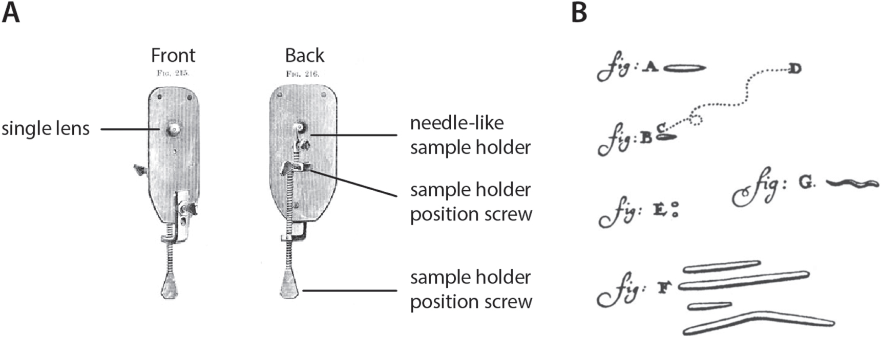
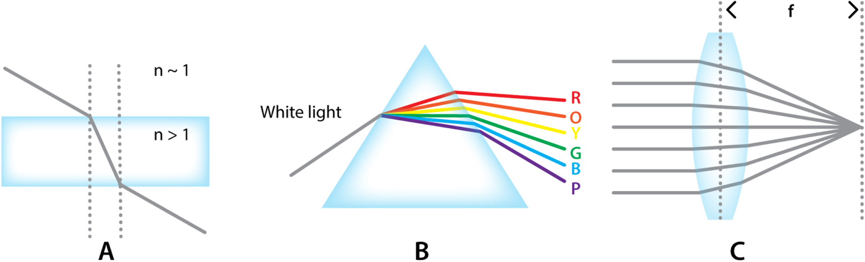
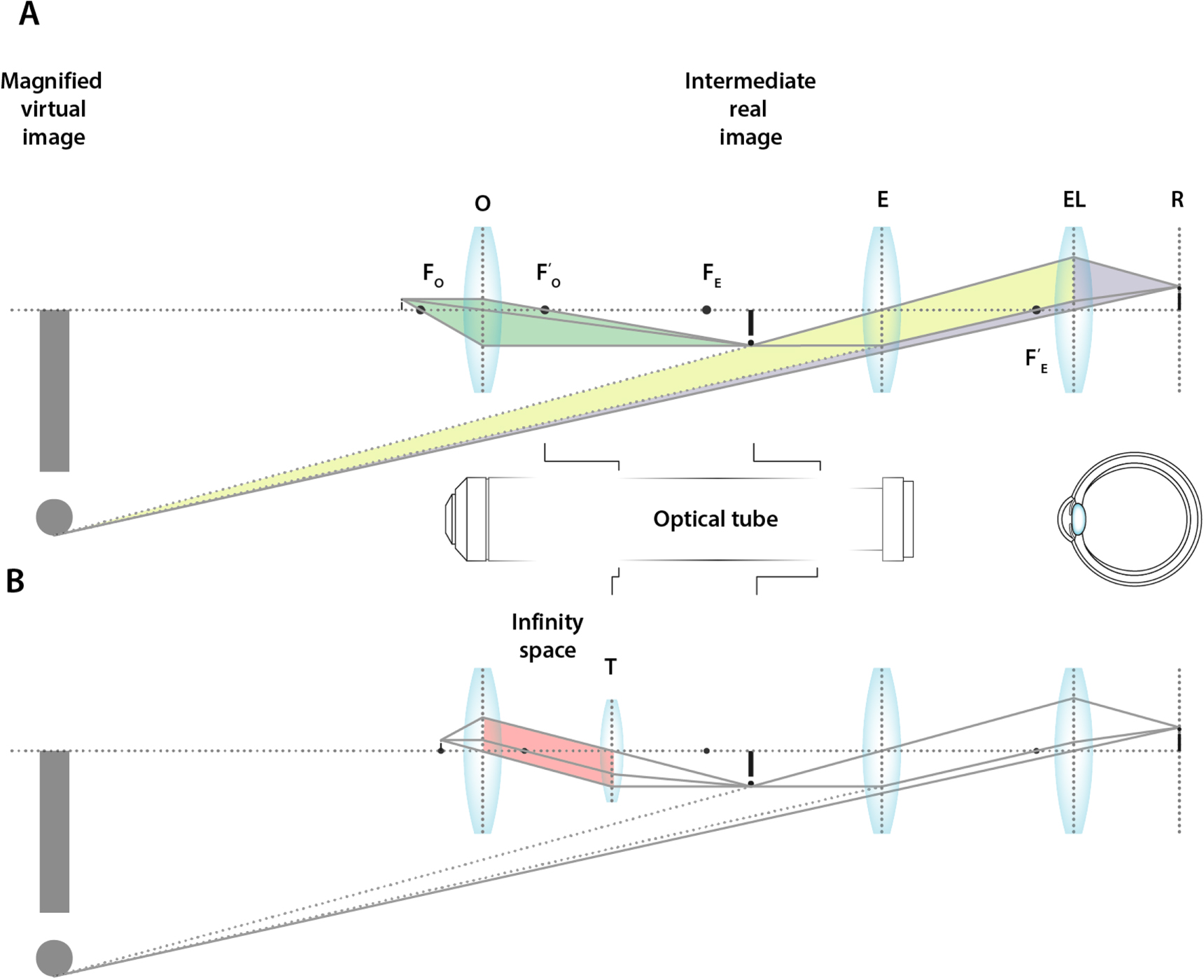
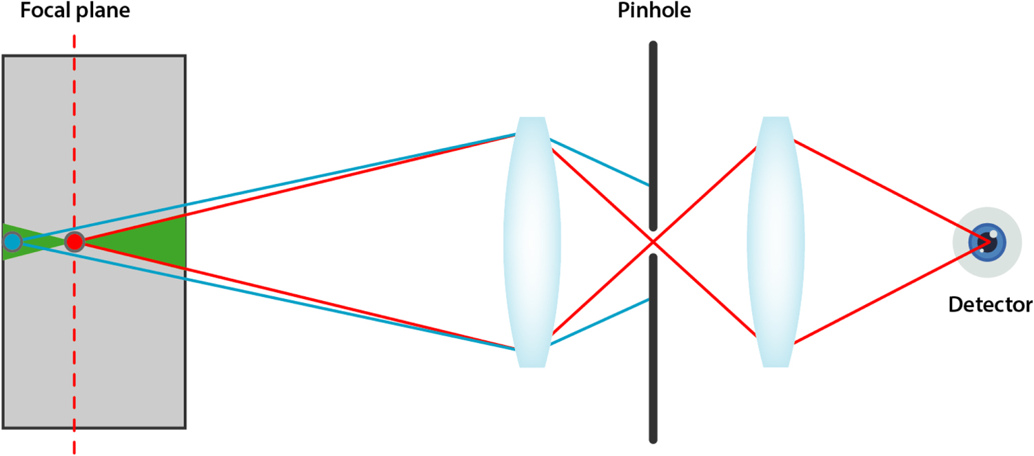
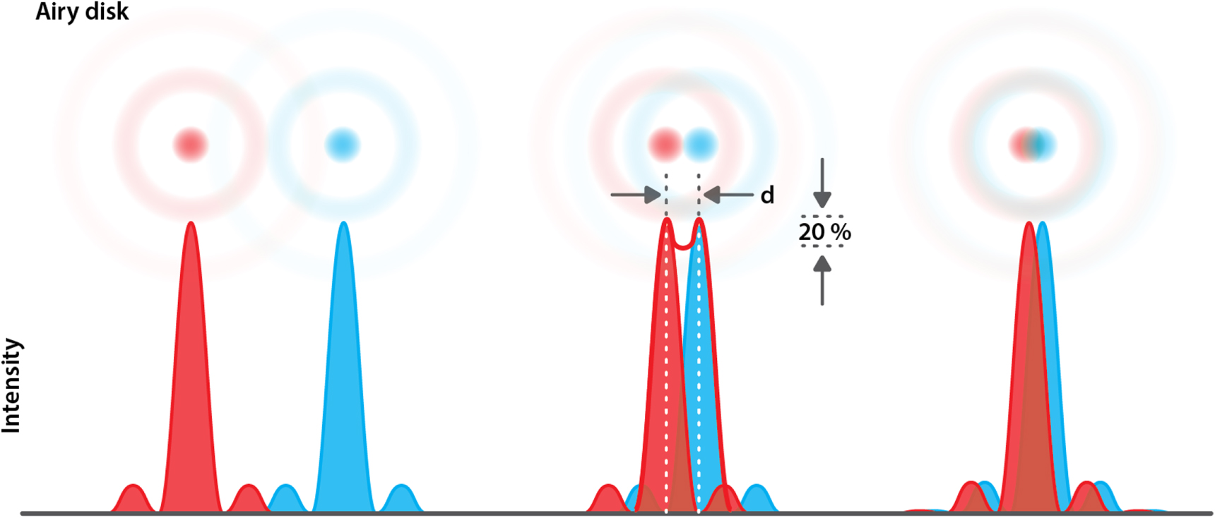
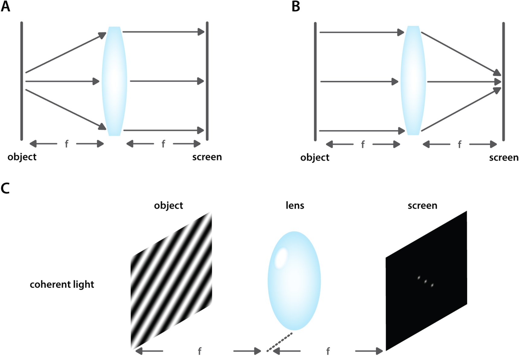
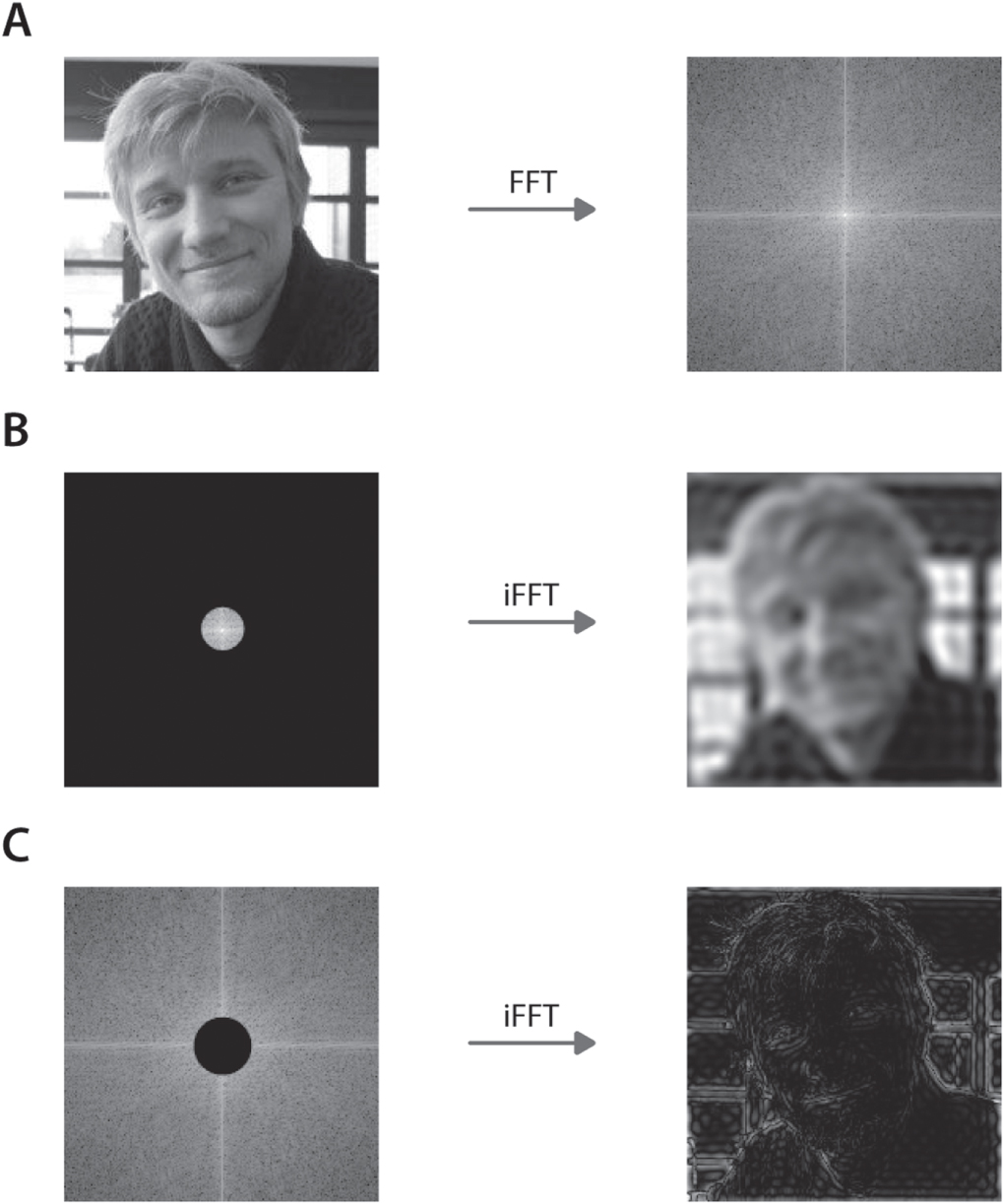
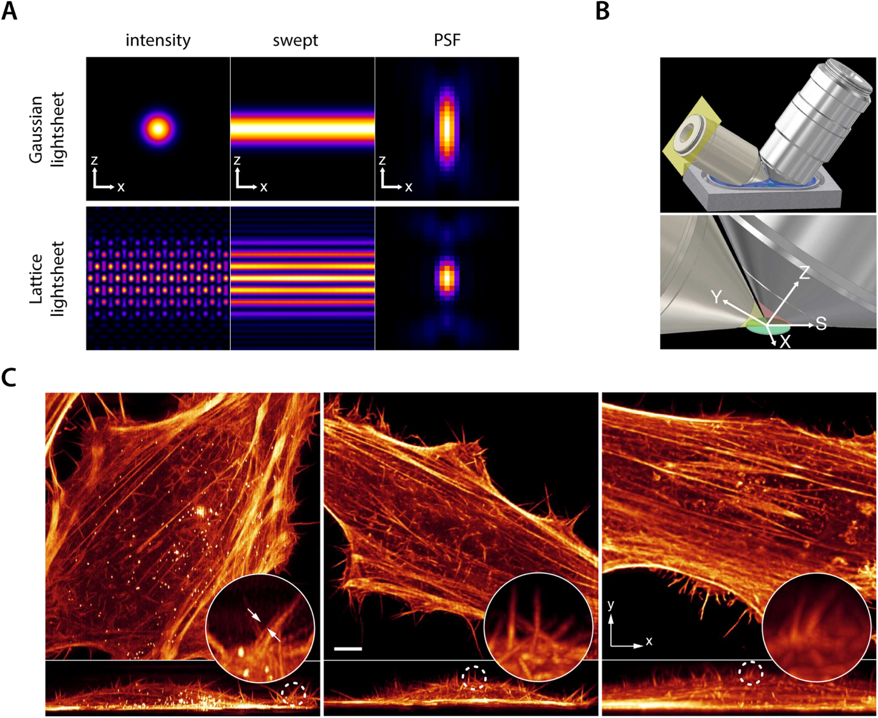
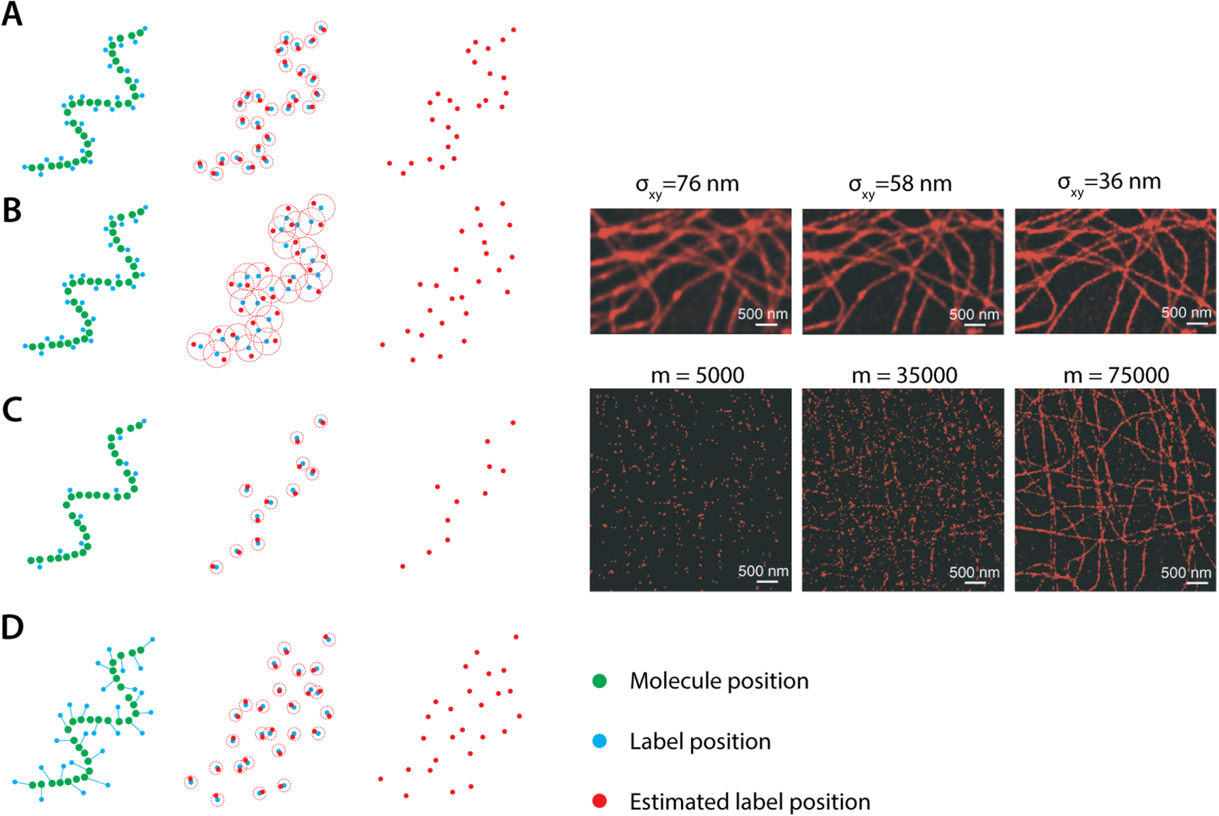
Figure 51. 3D pcSOFI of mitochondria in HeLa cells. Mitochondria were targeted by DAKAP target sequence, fused to Dronpa. Scale bar is 10 μm. Reproduced from Dedecker et al [203].
Download figure:
Standard image High-resolution image
Recently, multi-plane imaging was combined with SOFI to enable 3D imaging [210]. Rather than performing axially scanned nth order SOFI with 2D cross-cumulant calculation for each imaged plane, 3D cross-cumulants were calculated across the individual depth planes, effectively yielding virtual image planes that supplement the physically recorded data [210]. This provides a number of benefits. Most notably, the axial PSF does not need to be oversampled resulting in a reduction of the acquisition time and reduced photo bleaching [210].
A key recent development in SOFI imaging has been the visualization of genetically-encoded biosensors at sub-diffraction resolution [211, 212]. These biosensors can provided a space-and-time resolved picture of e.g. protein interactions or enzymatic activities, vastly expanding the range of questions that can be addressed. However, adding the biosensor functionality to an existing fluorophore typically requires compromises in the probe brightness or other spectroscopic properties, rendering SOFI an excellent technique to visualize these at super-resolution, especially for dynamic imaging.
Conclusions
Through the combination of sensitive cameras, with the ability to image single fluorophores, tailored probes which can be controllably switched between 'on' and 'off' states and powerful computers, capable of analyzing large sets of image data, SMLM has become one of the most powerful imaging tools in the biologists' toolbox. Modalities such as PALM and STORM are not only capable of delivering some of the highest resolving powers across all super-resolution modalities but also inherently lend themselves to quantify molecules of interest or measure their dynamics and interactions in biological contexts. To some extent, these advantages come at the cost of generally lower time-resolution when compared to approaches such as e.g. STED. Indeed, as sufficient localization events need to be accumulated and most fluorophores are typically in the dark state, acquisition times might become significant. Although easy to use commercial equipment exists, sample preparation can be complex as the use of specialized fluorophores becomes necessary and the labeling density is essential. Moreover, maintaining a favorable distribution of fluorophores between the 'on' and 'off' state generally implies use and optimization of specialized sample mounting media and some insight regarding photo chemical processes on the part of the user. Finally, like STED or SIM, SMLM might also be subject to limitations when it comes to image deep inside thick biological samples.
The large number of variations and extensions of the core SMLM concept enable the imaging modality to be judiciously adapted to the task at hand. In livePALM time resolution can be increased, at the expense of absolute resolution. Likewise, SOFI, which relies on the analysis of correlations in fluorescence intensity fluctuations rather than true single molecule localization, generally allows a larger fraction of emitters to reside in the 'on' state during imaging. A larger number of photons therefore contribute to each captured image, ultimately reducing the total time required for acquisition. In addition, SOFI imaging has broken new ground in its ability to dynamically image biosensor at sub-diffraction spatial resolution. Combination of SMLM with e.g. SPIM or Lattice light sheet illumination has enabled 3D imaging deep inside biological tissues. Exciting new concepts such as the recently developed MINimal photon FLUXes (MINFLUX) microscopy allow tracking of molecules at unprecedented spatiotemporal resolutions [213]. Finally, the quality of super-resolution images obtained in SMLM depends in no small part on the software used to detect and accurately localize point sources [214]. A plethora of algorithms exist, some of which might be optimized for speed, 2D or 3D localization or to deal with low signal to noise quality data whereas others are better suited to deal with datasets that where the condition of sufficient 'on' state sparsity could not be fulfilled [214]. An exhaustive review of these computational methods goes well beyond the scope of this manuscript but in depth reviews exist elsewhere [215].
General conclusions
This review aims to provide aspiring or even experienced life scientists a primer on the basic concepts of fluorescence microscopy and the operating principles of the major classes of super-resolution imaging modalities. This manuscript can serve to provide the necessary background to further explore applications of super-resolution microscopy in e.g. cell biology [216], prokaryotes [217], or eukaryotes [218].
Most of the discussed techniques are based on the same principle: by separating fluorescence emission in time, space, or both, additional information on the location of the emitter could be extracted, leading to higher resolution images. However, imaging resolution in super-resolution imaging is an elusive concept and might ultimately not be the single most important guideline when choosing the right super-resolution modality for a particular application.
In conventional microscopy, resolution is mostly treated within theoretical context of the Rayleigh Criterion. Still relevant today, it allows one to evaluate the resolving power of an optical system by simply imaging a sub-diffraction point emitter and determining the full width half-maximum (FWHM) of the ensuing PSF. When assessing the true resolution of experimentally obtained super-resolution images, it is commonplace to report the FWHM of a sufficiently small or narrow feature in the image such as tubulin or actin filaments [219]. Fourier spectrum analysis allows the spatial frequency bandwidth of an image to be determined which, as outlined previously is related to resolution. Demmerle et al provide an excellent evaluation of these approaches [219]. Fitting of a Gaussian profile to estimate FWHM in diffraction limited and SIM images provides very precise resolution estimates whereas this approach seems less suited for STED, where depletion often results in poorer signal-to-noise ratios for the acquired images and where PSFs might no longer be approximated by a Gaussian. This translates to higher uncertainty for the image resolution. In the case of SMLM, resolution is determined by localization precision as well as labeling density and the number of localizations. If this number is low, FWHM estimation might yield numbers that are close to the localization precision even though images acquired in these conditions might not necessarily be a good representation of the sample structure (figure 43) [219].
Fourier spectrum analysis and related approaches on the other hand might be affected by artefacts induced e.g. by the typically low SNR offered by STED or the limited number of orientations of the illumination pattern in SIM. It might be particularly inapplicable to SMLM as image reconstruction typically involves plotting a perfect Gaussian at each localized position. Such a Gaussian is inherently composed of an unlimited number of spatial frequencies [219]. Some of these issues might be addressed by more advanced frequency analysis approaches such as Fourier ring correlation analysis (FRC) [220] although there is evidence that this method might also be subject to unreliable estimates under certain conditions [120].
Therefore, one should always be careful to define exactly what a certain resolution estimate means. All techniques discussed have their advantages and disadvantages and it is to the user to decide which technique is the most appropriate in providing an answer to their research question. Co-localization questions might be best tackled by SMLM as it has the highest resolution, while highly dynamic systems or processes could benefit from STED based approaches. If ease of sample preparation is preferred over absolute resolution, SIM or SOFI could provide an excellent compromise. It all comes down to researchers matching their specific research question to the most appropriate super-resolution technique, as one flavor will not serve all. With commercial instrumentation becoming ever more attainable, along with standardized operating and sample preparation protocols, the different flavors of super-resolution microscopy are ready to be more widely adopted. As ever larger numbers of users come to terms with the concepts and techniques at hand, it can be envisioned that super-resolution microscopy will play a more central and prominent role in biological and medical research for many years to come.
Acknowledgments
K P F J would like to thank Industrieel Onderzoeksfonds (IOF) for grant C32/16/005. K P F J would additionally like to thank FWO Flanders for post-doctoral scholarships 12C2814N and 12C2817N.
Conflict of interest statement
The authors declare that no conflicting interests exist.